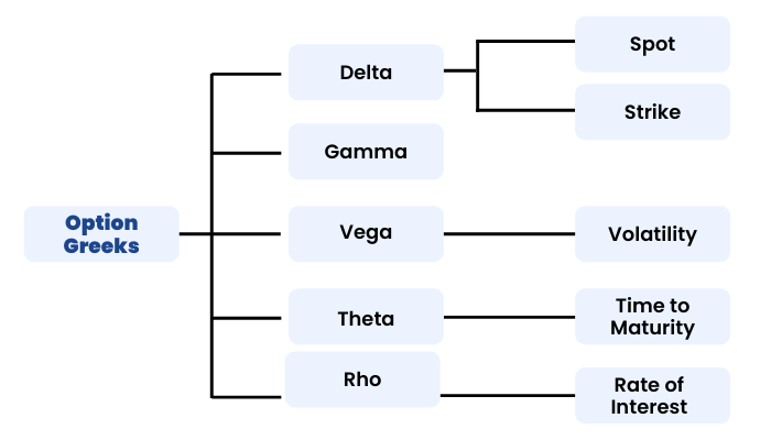
Option Greeks
Introduction To Greeks
For a successful options trade, there are a number of forces which have to work in the favour of the trader. These forces are called ‘The Option Greeks’. These forces influence the option prices in real time. These forces not only affect the premiums but also affect each other.
The sensitivity of option premium to each of these factors is known as Option Greeks.
These Greeks are Delta, Gamma, Theta, Vega and Rho. Option Greeks gives us a thorough understanding of a portfolio’s position. We have already learnt the basics of the Option Greeks in our Basics of Options Module. Let us now elaborate on the same.
Black Scholes Model
Before we move to different option greeks, let us learn a popular model called ‘The Black Scholes Model’ that is used to calculate option value.
The Black Scholes model, also known as the Black-Scholes-Merton (BSM) model, is a mathematical model for pricing an options contract. The Black-Scholes Merton (BSM) model is a differential equation used to solve for options prices. The model won the Nobel prize in economics. It's used to calculate the theoretical value of options using current stock prices, expected dividends, the option's strike price, expected interest rates, time to expiration and expected volatility.
The formula, developed by three economists—Fischer Black, Myron Scholes and Robert Merton—is perhaps the world's most well-known options pricing model.
The Black-Scholes model makes certain assumptions:
- The option is European and can only be exercised at expiration.
- No dividends are paid out during the life of the option.
- Markets are efficient (i.e., market movements cannot be predicted).
- There are no transaction costs in buying the option.
- The risk-free rate and volatility of the underlying are known and constant.
- The returns on the underlying asset are normally distributed.
While the original Black-Scholes model didn't consider the effects of dividends paid during the life of the option, the model is frequently adapted to account for dividends by determining the ex-dividend date value of the underlying stock.
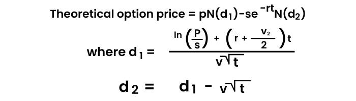
The variables are:
p= stock price
s= strike price
t= time to expiry
r= current risk-free interest rate
v= volatility measured by annual standard deviation
ln= natural logarithm
N(x)= cumulative normal density function
The model assumes stock prices follow a lognormal distribution because asset prices cannot be negative (they are bounded by zero).
Introduction To Delta
Let us start with the first option-greek ‘Delta.’
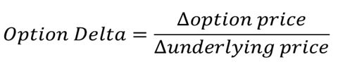
Delta measures the change in option price for a unit change in the price of underlying. So, if an option has Delta 0.47 it shows that if the underlying price changes by ₹1, the option price will change by ₹0.46.
Delta varies from a range of -1 to 1. For call options, delta is 0 to 1 and for put options, delta ranges from -1 to 0.
Let’s discuss some important points with respect to Delta.
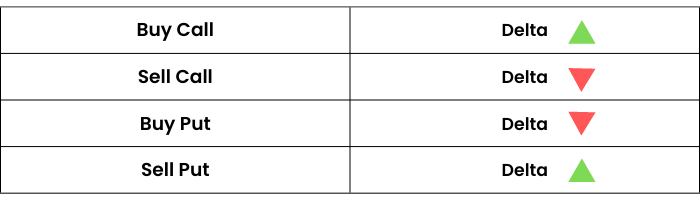
- The Delta of Call Option is always positive and the Delta of Put Option is always negative.
- When you buy Call Option, Delta is positive and when you sell Call Option, Delta is negative.
- When you buy Put Option, Delta is negative and when you sell Put Option, Delta is positive
- When you buy Call Option, Positive Delta multiplies by Positive quantity (quantity is considered positive when we go long on option), hence gives positive portfolio Delta. This signifies that buying Call Option means Bullish position.
- When you sell Call Option, Positive Delta multiplies by negative quantity (quantity is considered negative when we go short on option), hence gives negative portfolio Delta. This signifies that selling Call Option means Bearish position.
- When you buy Put Option, Negative Delta multiplies by Positive quantity, hence gives negative portfolio Delta. This signifies that buying Put Option means Bearish position.
- When you sell Put Option, Negative Delta multiplies by Negative quantity, hence gives Positive portfolio Delta. This signifies that selling Put Option means Bullish position.
Delta’s Relationship With Spot And Strike Price
Let’s learn more about the effect of different factors on Delta.
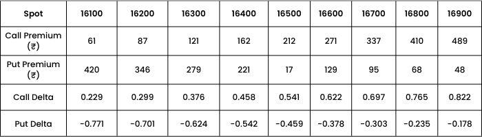
The table below shows how Delta changes with respect to change in SPOT PRICE, given the other factors are constant. Let’s find out the same for a 16500 strike Call and Put option, assuming the volatility to be 17% and days to expiry 17 days.
Note: All the premium and Greek figures in this table (and the upcoming ones), have been derived using Black Scholes options pricing calculator.
Observations:
We can clearly observe that as spot price increases from 16100 to 16900, call premium increases (from ₹61 to ₹489) and put premium decreases(from ₹420 to ₹48). Similarly, call Delta increases and put Delta decreases. Thus concluding that call Delta has a positive relationship with Spot price whereas Put Delta has a negative relationship.
Now let’s find out how Delta behaves with respect to change in STRIKE PRICE, assuming the Spot price to be 16500, days to expiry 17 and volatility at 17%.
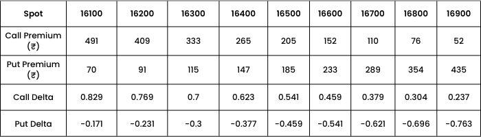
Observations: As Strike price increases,
- Call premium decreases from 491 to 52
- Put premium increases from 70 to 435
- Call Delta decreases.
- Put Delta increases.
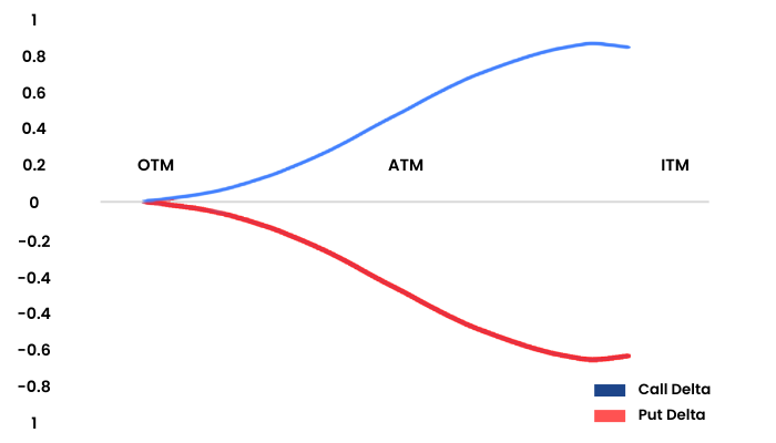
In this graph, we can see that the X axis shows the moneyness of the option. The blue Delta line is flattish at the OTM near zero. When the spot moves from OTM to ATM the Delta also starts to pick up and remains in the range of 0 to 0.5. When the spot moves from ATM to ITM, the Delta moves beyond the 0.5 mark and starts to flatten out as it hits the value of 1. A similar characteristic is shown by the red line Put Delta.
This means that when you are buying an ITM option it is as good as buying the underlying itself.
To compute the exact Delta of an option, one can always use the Black Scholes option pricing calculator.
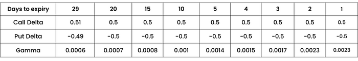
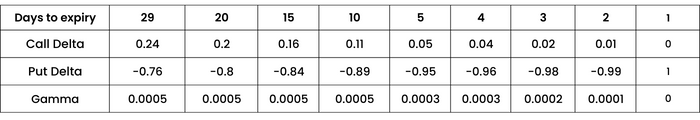
Delta And Time To Expiry
Now we will understand Delta with respect to change in Days to Expiry:
An option’s Delta changes as one trading day passes. This is often called “Delta Decay”.As the expiration is nearing, the time value portion of an option is declining. This causes the Delta of ITM options to increase (i.e. ITM option’s Delta gets closer to 1 for Calls or to -1 for Puts) and the Delta of OTM options to decrease (i.e. OTM option’s Delta gets closer to 0).
Assuming the Spot price to be 17500 and volatility at 17%, let us figure out the behavior of ITM, ATM and OTM options and their Deltas.
At The Money Strike 17500
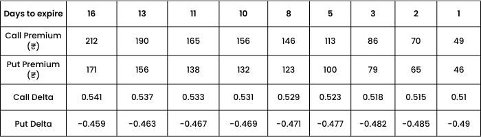
Observations: As days to expiry decreases,
- Both Call and Put premiums decrease.
- ATM option approaches to 0.5 for call and -0.5 for put.
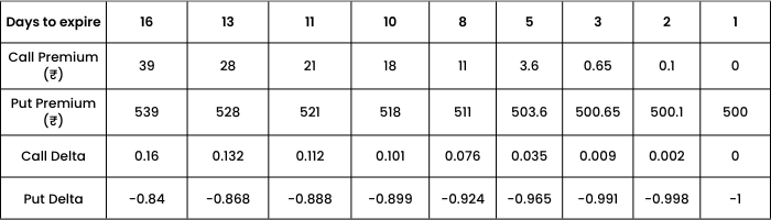
Strike 17000 where call option is ITM and put option is OTM

Here, as the days to expiry decreases,
- ITM Call Option approaches to 1.
- OTM Put option approaches to 0.
Strike 18000 where call option is OTM and Put option is ITM
Again, as we are nearing maturity, or as days to expiry decreases, we see
- OTM Call Option approaches to 0.
- ITM Put option approaches to -1.
One should avoid buying deep OTM options because the Deltas are really small and the underlying has to move by large value to work in favor. However, for the very same reason, selling deep OTM options makes sense (we shall discuss this when we learn Theta).
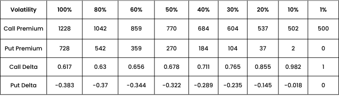
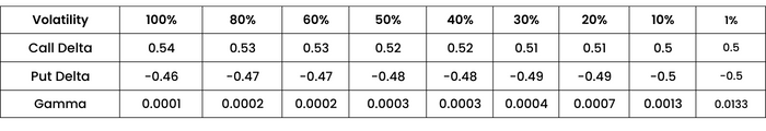
Delta And Volatility
Next, we will learn Delta with respect to change in volatility:
Changes in volatility will change Delta. Even though the stock price doesn’t move, Delta will change when there are changes in volatility. However, for the ATM options, the Delta is relatively unaffected to changes in volatility. This means ATM options will have Deltas close to 0.5 (assuming other factors are constant).
Let’s look at the table given below where Spot is 17500 and days to expiry is 14.
AT THE MONEY STRIKE 17500
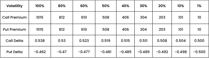
Observations: As Volatility decreases,
- Both Call and Put premium decreases.
- Call Delta and Put Delta both approach 0.5 and -0.5 respectively.
Let us figure out the same for ITM/OTM strikes. First let us take a strike, here the call option is ITM and obviously the put option for the same strike is OTM.
STRIKE 17000 where call option is ITM and put option is OTM
As volatility decreases, both Call and Put premium decreases. However,
- ITM Call Option approaches to 1.
- OTM Put option approaches to 0.
Now let us calculate the same for the strike where Put option is ITM and call option is OTM.
STRIKE 18000 where call option is OTM and put option is ITM
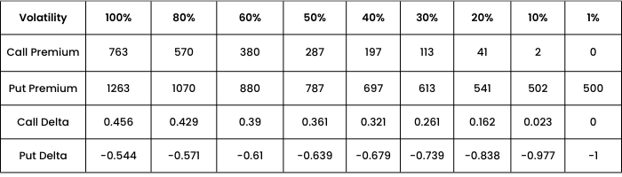
The observation here is the same that both call and put option premium decreases with a decrease in volatility. Just now the call option is OTM, so its delta approaches 0 while, Put option being ITM, its delta approaches -1.
We see that in contrast to the ATM, the ITM or OTM option Delta is more sensitive to changes in volatility.
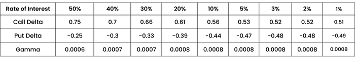
Lastly, let’s try to figure out the relationship of Delta with respect to the Rate of Interest.
Assuming spot to be at 17500 and taking ATM options, days to expiry 14 days and volatility to be 17%.
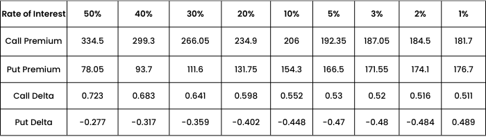
Observations: As Rate of Interest decreases,
- Call premium decreases and Put premium increases.
- Call Delta decreases and Put Delta increases.
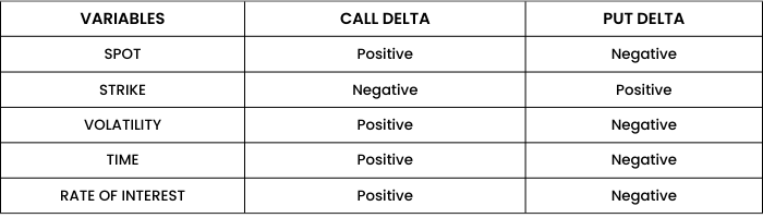
Let us now sum up the relationship of Delta with different variables.
Delta Adds Up
In this section, we will learn an interesting characteristic of Delta is that it can be added up. We have already learnt that the Delta of a futures contract is 1. Now assume that I hold an ATM call option which has a Delta of 0.5. This in other words means that I am holding a half futures contract. Given this, if I hold 2 ATM options then it is as good as holding one future contract because 2 options of Delta 0.5 add up to 1.
Case 1. Nifty spot at 16000, trader has 3 different call options.
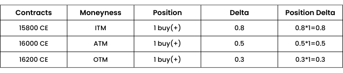
The positive sign in the position column indicates a long/ buy position of call, hence positive Delta. So, the total Delta of the portfolio will be (0.8+ 0.5 + 0.3) = ₹1.6
This means that if Nifty moves up by 1 point, the trader will gain ₹1.6 and if Nifty moves down by 1 point, he will suffer a loss of ₹1.6.
So, if nifty moves up by 50 points, the combined position is expected to move by (50*1.6) = ₹80
Case 2.Nifty spot at 16000, trader holds a combination of call and put options.
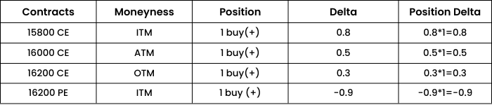
The Put option shows a positive position, which means it has been bought or the trader is long on that option. However, Put option has a negative Delta, hence (+1 * -0.9) = -0.9 .The Delta of the put position is negative.
Therefore, the combined Delta of the portfolio is (0.8 + 0.5 + 0.3 + 9- 0.9) = 0.7
This implies that if Nifty moves by 1 point, the total combined position will have an effect of 0.7 points. So, if Nifty moves up by 50 points, the profit (because positive Delta means gaining with price increase) will be 50*0.7 = ₹35
An important point to keep in mind is, Deltas of call and put can be added as long as they belong to the same underlying.
Let us consider one more example to explain the Delta:
Case 3 Nifty is at 16000
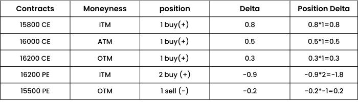
When the trader is selling a put, he is getting a positive Delta (because we know negative quantity into negative delta gives positive delta result). So the combined Delta of this portfolio is 0.8 + 0.5+ 0.3 + (-1.8) + 0.2 = 0
This creates a Delta neutral portfolio for him as the combined Delta is zero. So this portfolio has no impact with the spot price movement. However, Delta keeps on changing because of time and volatility, so a portfolio can be Delta neutral only for a moment. We will learn more about Delta hedging and Delta neutral in upcoming chapters.
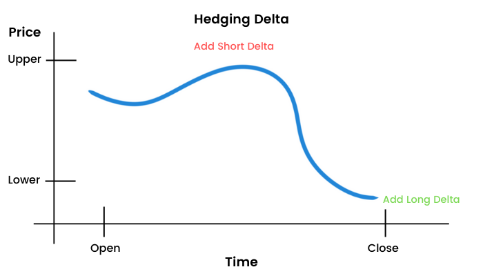
Delta Hedging
Delta hedging is an option trading strategy that aims to reduce, or hedge, the directional risk associated with price movements in the underlying asset.
For e.g.: Imagine I hold 500 shares of XYZ Ltd @ ₹100. When the stock price will go up, I’ll gain and when the stock price will go down, I’ll lose.
To protect myself from the downside directional risk, I will try to offset my risk by creating a negative Delta (i.e. by taking a bearish position). Suppose, a call option of strike 100 is trading at ₹3 and has a Delta of 0.55.
I want to sell 300 call options. So, now Delta of my option position is-
300* (-0.55) =-165 (Delta is negative when we sell call option)
Now, when the stock price goes up by ₹20, profit on the stock position is (500*20)= ₹10000/-
Premium received for selling call option = (300*3)= ₹900/-
Whereas loss on call option is (0.55*20*300)= ₹3300/-
So the net profit will be 10000+900-3300= ₹7600/-
If the stock price goes down by ₹20, loss on the stock will be (500*20)= ₹10000/-
Premium received for selling call option= ₹900/- (Maximum profit for selling option is the premium received)
So the net loss will be 10000-900= ₹9100/-
Here we can see that I have hedged myself partially against the downward price risk, where instead of losing ₹10000/- , I lost ₹9100/-. This is called Delta hedging, where I try to take advantage of my fear. This has just partially helped me cover my risk.
However, we can sell more call options to offset the risk to a larger extent or create a zero Delta position. This is called Delta neutral. A portfolio is just momentarily Delta neutral because the Gamma and Delta of an option keeps on changing. So we have to keep on adjusting Delta with different and continuous trades. We shall learn more about it in upcoming chapters.
Question to ponder over?
Have you tried to find out the Delta of an option when the volatility is 10,000%?
Answer: All Delta turns to 1 in such extreme situations.
AMAZING FACT
There is yet another way to interpret Delta.
“Delta is the probability of the option contract being in-the-money at expiration”. This is not a theoretical definition of Delta but has helped me to understand more about its behavior.
For example,
Q) Why for ITM options, for the same strike price, the longer days to expiration, Delta is lower?
A) More time to move means less likelihood of the option still being in-the-money at expiration; this translates into a smaller Delta.
Q) Why for OTM options, for the same strike price, the longer days to expiration, the Delta is higher?
A) If you’re buying OTM options, you need time for the stock to move up to the strike price. In other words, there’s a much higher probability of the underlying finishing ITM for the (longer to expiration) option than for the (nearer to expiration) option; Delta reflects that probability.
Hope this can help you to understand Delta better too !!
Introduction To Gamma
The next option-greek that we will learn is ‘Gamma.’
Gamma measures the change in Delta with respect to per unit change in underlying. If Gamma value is 0.0008, it shows that my next move in Delta will be 0.0008 if underlying changes by 1. So Gamma shows what will be the next change in Delta with respect to change in underlying.
Important Points:
- The Gamma of an option is always positive. Positive Gamma means that the Delta of long calls will become more positive and move toward +1.00 when the stock price rises, and less positive and move toward 0 when the stock price falls. Long Gamma also means that the Delta of a long put will become more negative and move toward –1.00 if the stock price falls, and less negative and move toward 0 when the stock price rises. For a short call with negative Gamma, the Delta will become more negative as the stock rises, and less negative as it drops.
- The Gamma of Call and Put Option is same. Because Gammas influence Deltas of calls and puts in the same way, expressing their probability of finishing in the money after a change in price in the underlying.
- Gamma is highest at ATM and decreases as Spot price moves away.
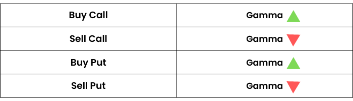
When you buy Call Option, Positive Gamma multiplies by Positive Quantity (positive quantity because going long on option), hence gives Positive Portfolio Gamma. This signifies that buying Call Option means Long Gamma Position.
When you sell Call Option, Positive Gamma multiplies by Negative Quantity (negative quantity because going short on option), hence gives Negative Portfolio Gamma. This signifies that selling Call Option means Short Gamma Position.
When you buy Put Option, Positive Gamma multiplies by Positive Quantity, hence gives Positive Portfolio Gamma. This signifies that buying Put Option means Long Gamma Position.
When you sell Put Option, Positive Gamma multiplies by Negative Quantity, hence gives Negative Portfolio Gamma. This signifies that selling Put Option means Short Gamma Position.
If Gamma is small, Delta changes slowly. However, if the absolute value of Gamma is large, Delta is highly sensitive to the price of the underlying. Let us now take a look at how different parameters affect Gamma in our upcoming chapters.
Gamma’s Relationship With Spot And Strike Price
Gamma with respect to change in spot price:
The table below shows how Gamma changes with respect to change in SPOT PRICE, given the other factors are constant. Let’s find out the same for a 16500 strike Call and Put option, assuming the volatility to be 17% and days to expiry 17 days.

Observations:
We can clearly observe that as spot price increases from 16100 to 16900, call premium increases and put premium decreases. Gamma is highest at ATM (here 0.0008) and decreases as spot price moves away in either direction. When Nifty slides down to 16100, gamma too goes down to 0.0007. When Nifty goes up to 16900, gamma still goes down to 0.0005.

The Gamma peaks when the option hits ATM status. This implies that the rate of change of Delta is highest when the option is ATM. In other words, ATM options are most sensitive to the changes in the underlying. Also, since ATM options have the highest Gamma – avoid shorting ATM options.
Let us now evaluate how Gamma changes with respect to change in other variables.
Gamma with respect to change in Strike Price:
Given the spot 16500, volatility at 17% and days to expiry 17 days.

We can see that the Gamma is highest (0.0008) at the ATM(13500) and decreases as Nifty moves away on either side. When Nifty comes down to 15500, gamma too slides down to 0.0001 and when Nifty moves up to 17500, gamma still reduces to 0.0002. This explains why gamma has a bell curve.
Gamma And Time To Expiry
Gamma with respect to change in Days To Expiry.
Assuming Spot to be 16500, volatility 17%, let us find out how gamma changes for ATM option 16500,
As days to expiry decrease, call Delta decreases and put Delta increases. They both tend to move towards 0.5 and -0.5 respectively. However Gamma increases, showing the high sensitivity of ATM options.
Gamma values for options with nearer time to expiration differ more significantly along various strike prices, as compared to those with further time to expiration. The further the time to expiration is, the smaller the difference in gamma values across different strike prices will be.
Now let us check the same for strike 16000 where call is ITM and put is OTM

For, 16000 strike, or ITM call Delta moves towards 1 and OTM put Delta towards 0. The Delta being less sensitive on either side, Gamma tends to move towards zero.
Now for strike 17000 where call is OTM and put is ITM
Similarly, for ITM Put, the Delta moves towards 1, while for OTM call Delta is 0. Gamma still moves towards Zero, showing no sensitivity in either direction.
The Gamma value is also low for ITM options. Hence for a certain change in the underlying, the rate of change of Delta for an ITM option is much lesser compared to ATM option. However, do remember the ITM option inherently has a high Delta. So while ITM Delta reacts slowly to the change in underlying (due to low Gamma) the change in premium is big (due to high base value of Delta).
Learnings!
- Delta changes rapidly for ATM options.
- Delta changes slowly for OTM and ITM options.
- Never short ATM or ITM option with a hope that they will expire worthless upon expiry
- OTM options are great choices for short trades assuming you intend to hold these short trades up to expiry wherein you expect the option to expire worthlessly.
Gamma And Volatility
Gamma with respect to change in volatility:
When volatility is low, the Gamma of At-the-money (ATM) options is high, while the Gamma for deep In-the-money(ITM) or Out-of-the-money (OTM) options approaches 0. This phenomenon arises because when volatility is low, the time value of such options is low, but it goes up dramatically as the underlying stock price approaches the strike price.
When volatility is high, Gamma tends to be stable across all strike prices. This is due to the fact that when volatility is high, the time value of deep In or Out-of-the-money options is already quite substantial. Thus, the increase in the time value of these options as they move nearer to At-the money will be less dramatic and hence the low and stable Gamma.
Keeping constant, the strike 16500, spot at 16500 and days to expiry 17, let us calculate how changes in volatility changes the gamma of an option.
As volatility increases, there will be an increase in the price of the options and vice versa. Thereby, we can see that as volatility decreases, call Delta decreases and put Delta increases.
The Gamma too increases. High Gamma values mean that the option tends to experience volatile swings.
GAMMA WITH RESPECT TO CHANGE IN RATE OF INTEREST RATE
Strike 16500 spot 16500 days to expiry 17 Volatility 17%
As the interest rate decreases, we can find Gamma increasing for the ATM call and put.
Important Properties Of Gamma
Let us summarize the relationship of Gamma with different factors:

A good way to think of Gamma is the measure of the stability of an option’s probability. If Delta represents the probability of being in-the-money at expiration, Gamma represents the stability of that probability over time.
Ready to unlock the secrets of gamma? Enroll now for our Masterclass on 7 Profitable Options Trading Strategies!
If you're an option buyer, high Gamma is good as long as your forecast is correct. That's because as your option moves to ITM, Delta will approach towards 1 more rapidly. But if your forecast is wrong, it can drastically affect your position by rapidly lowering your Delta.
If you're an option seller and your forecast is incorrect, high Gamma is an enemy. That's because it can affect your position to work against you at a more accelerated rate- if the option you've sold moves to ITM. But, if your forecast is correct, high Gamma is your friend since the value of the option you have sold will lose value more rapidly.
Introduction To Theta
‘Theta’ is the next option-greek that we will understand in this chapter.
Theta measures the change in options price per day change in time to expiry. It can also be referred to as the time decay of an option. This means an option loses value as time moves closer to its maturity, considering other variables constant. Theta is generally expressed in negative numbers and can be thought of as the amount by which an option’s value declines every day. If days Theta is -3.87 that signifies that for the next day the options price will decrease by 3.87.
Option premium = Intrinsic value + Time Value
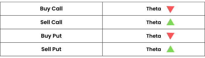
- Theta of an option is always negative.
- Theta of call and put option is same. (if interest rate is not considered into calculation)
- Theta is highest at ATM and decreases as Spot moves away.
When we buy Call option, negative Theta multiplies by positive quantity, hence gives negative portfolio Theta. This signifies that buying call option means short Theta position.
When we sell Call option, negative Theta multiplies by negative quantity, hence gives a positive portfolio Theta. This signifies that selling call option means long Theta position.
When we buy Put option, negative Theta multiplies by positive quantity, hence gives negative portfolio Theta. This signifies that buying put option means short Theta position.
When we sell Put option, negative Theta multiplies by negative quantity, hence gives a positive portfolio Theta. This signifies that selling put option means long Theta position.
Let’s assume the Nifty spot at 16500, a trader buys a Nifty 16800 call option. What is the likelihood of this call option to expire ITM in the next 29 days? The chance of Nifty moving over 300 points in the next 29 days is quite high.
Now if the trader has only 14 days left to expiry? Now the chance of nifty reaching that mark is still reasonable, so the chances of option expiring ITM is still high, although not very high.
Now if I consider 5 days, I would say that chances of nifty reaching 16800 is low.
And when there is 1 day left to expiry, I would say the chances that Nifty will reach 16800 is very low.
So, the more time for expiry the likelihood for the option to expire ITM is higher.
Now, if a trader sells an option, he receives the premium for it. He is well aware that he carries an unlimited risk and limited reward potential (which is limited to the premium he receives). This is also possible only if the option expires worthless or OTM.
Next, in our upcoming sections, we will study the effect of different parameters on Theta.
Theta’s Relationship With Spot And Strike Price
Theta with respect to change in spot price:
Assuming the strike to be 16500, days to expiry 17 days and volatility 17%


When the stock price is very low, Theta is close to zero. For an ATM option, Theta is large and negative. As stock price increases,Theta again tends to move towards zero, but stays negative.
Theta with respect to change in strike price:
Assuming spot to be 16500, days to expiry 17 and volatility 17%

Value of Theta increases as the option moves from OTM to ATM and decreases as the option moves from ATM to ITM. In other words, Theta is at its peak at ATM and decreases as Nifty moves away.
Theta And Time To Expiry
Theta with respect to change in days to expiry:
Spot constant @ 16500, volatility 17%
Theta is higher for shorter term options, especially ATM options. This is pretty obvious as such options have the highest Time value and thus have more premium to lose each day.
Conversely, Theta goes up dramatically as options near expiry have the highest time decay.
Theta And Volatility
Theta with respect to changes in volatility:
In general, options of highly volatile stocks have higher Theta than those which are less volatile. This is because the time value premium on these options is higher, and so they have more to lose each day.
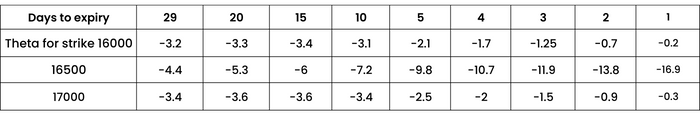
Let us consider Spot at 16500, days to expiry 17

From the table we can see that regardless of the option’s strike price (ATM/ITM/OTM), Theta always increases as Volatility increases. Like for strike 16500, Theta increases from 0.3 to 33 as volatility increases from 1 % to 100%.
Please note that negative sign, which means losing the time value, is ignored when doing the comparison.
As can be seen, for all the three options with different volatility, Theta always behaves the same way, i.e. Theta of ATM options is always higher, and it gets lower as it moves towards deep ITM or OTM.
However, a decrease in Theta as the option moves from ATM towards deep OTM/ITM will be much bigger for options with higher volatility as compared to options with lower volatility.
This is understandable because options with higher volatility will contain more time value than options with lower volatility. Since Theta decreases due to the passage of time, it will naturally be higher for options with higher volatility as it has more time value to lose compared to options with lower volatility.
Important Properties Of Theta
Theta relationship in a nutshell:

Rho
The next option-greek that we will study is ‘Rho.’
Rho measures the change in options price with unit change in rate of interest. If rho for put options is -3.8 that signifies that for each unit increase in interest rate, put option price will decrease by 3.8.
- Rho is always positive for the call option and negative for the put option.
- Rho for call and put is different.
- Rho is the highest at ATM and decreases as the spot moves away.
Unlock success in options trading with 'Rho'! Enroll now for our Masterclass on 7 Profitable Strategies.
As you might ask, "Why do interest rates impact option prices?"
It has to do with the cost of carrying the position over time. Pricing models take into consideration the cost of capital (or proceeds from short sales) used to offset risk.
The higher the price of the stock and the longer time until expiration generally means a greater sensitivity to changes in interest rates (higher absolute Rho values).
Rho is not of much importance in the Indian market because only short term options are liquid. It is more useful for people who trade in OTC long term contracts.
Introduction To Vega
We will learn the option-greek ‘Vega’ in this section.
Vega measures the change in option price per unit change in Volatility. If the absolute value of Vega is high, the portfolio’s value is very sensitive to small changes in volatility. However, if the absolute value of Vega is low, volatility changes have relatively little impact on the value of the portfolio. A Vega value of 6.87 shows that for every unit increase in volatility, option price will increase by 6.87.
- Vega of an option is always positive.
- Vega of call and put is same.
- Vega is the highest at ATM and decreases as the spot moves away in either direction (bell shaped).
Impact of Vega on a Portfolio of Options:
When you buy Call option, positive Vega multiplies by positive quantity, hence gives positive portfolio Vega which signifies that buying call option means long Vega position.
When you sell Call option, positive Vega multiplies by negative quantity, hence gives negative portfolio Vega which signifies that selling call option means Short Vega position.
When you buy Put option, positive Vega multiplies by positive quantity, hence gives positive portfolio Vega which signifies that buying put option means long Vega position.
When you sell Put option, positive Vega multiplies by negative quantity, hence gives negative portfolio Vega which signifies that selling put option means Short Vega position.
When thinking about Vega, we have to remember that expected volatility (implied volatility) is a reflection of price action in the options market. When options are bought by traders, expected volatility will increase. When options are being sold, expected volatility will decrease. With that said, when being long on options, we want the price of the option to increase. When being short on options, we want the price of the option to decrease.
That is why long options have positive Vega, and short options have negative Vega.
An increase in expected volatility will benefit the long option holder, as that indicates an increase in option pricing, hence the positive Vega assignment. A decrease in expected volatility will benefit the short option holder, as that indicates a decrease in option pricing, hence the negative Vega assignment.

When volatility increases, the stock/index price starts swinging heavily. To put this in perspective, imagine a stock is trading at ₹200; with an increase in volatility, the stock can start moving anywhere between ₹180 and ₹220 very quickly. So when the stock hits ₹180, all PUT option writers will start panicking as the Put options now stand a good chance of expiring In the money (ITM). Similarly, when the stock hits ₹220, all CALL option writers would start panicking as all the Call options now stand a good chance of expiring In the money (ITM).
Therefore irrespective of Calls or Puts when volatility increases, the option premiums have a higher chance to expire in the money.
Next, in our upcoming sections, we will study the effect of different parameters on Vega.
Vega’s Relationship With Strike Price
Changes in Vega with respect to change in Strike Price
Assuming spot to be at 16500, days to expiry 17 and volatility at 17%

As strike price increases, Vega is at its peak at ATM and decreases as the spot moves away in different directions.

Vega And Time To Expiry
Changes in Vega with respect to change in days to expiry
Assuming spot at 16500, volatility 17%

For all the options with different time to expiration, Vega always behaves the same way i.e. Vega of ATM options is always higher than deeper ITM and OTM options.
This makes sense because ATM options have the highest time value component, and a change in expected volatility will only affect the time value portion of the option. In a comparison between ITM and OTM options, volatility changes will have a greater effect on OTM options than on ITM options. This is because OTM options are comprised of only time value while ITM options are comprised of intrinsic value plus time value. The deeper the ITM options, the smaller the portion of time value it will have.

Volatility
Earlier, we learned about the option-greek Vega that measures the change in option price per unit change in volatility. But what exactly is volatility?
Volatility is a rate at which the price of a security increases or decreases for a given set of returns. It is measured by calculating the standard deviation of the annualized returns over a given period of time. It shows the range to which the price of a security may increase or decrease.
Let us consider an example to understand volatility better.
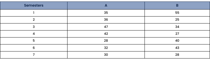
There are 2 students A and B and the table below shows the marks they have obtained in their last 7 semesters.
I am supposed to choose a student for a competition, who will be able to score at least 27 points.
Situation 1
Let us add up all the scores and see who scored the most
A=35+36+47+42+28+32+30= 250
B=55+25+34+27+40+43+28= 252
So, in this situation we can choose B as the total score is 252 (greater than A’s score)
Situation 2
Let us consider the mean or average for both the students
A=250/7= 35.7
B= 252/7= 36
So from this perspective also, I will choose B over A because his average is higher.
But we are not sure who will be able to score at least 27 points.
So let’s calculate the deviation from mean for each student and each semester.
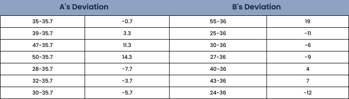
Now let’s further calculate another variable called variance. It is the sum of the squares of the deviation divided by the total number of observations.
So, variance= [(-0.7)^2 + (3.3)^2 + (11.3)^2 + (14.3)^2 + (-7.7)^2 + (-3.7)^2 + (-5.7)^2] / 7
=449/7
=64
Further, we will calculate Standard Deviation as √ of variance
= SQRT (64)
= 8
Similarly, B’s standard deviation comes to 10.75
Standard Deviation or the SD represents the deviation from the average. To forecast how much A and B will score in the next semester, we need to add and subtract SD from their average.
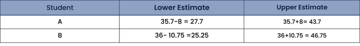
From these calculations, we can easily interpret that A is likely to score from 27.7 to 43.7 while B is likely to score 25.25 to 46.75. B has a wide range of scores because of which it is difficult to interpret whether he’ll be able to score at least 27. He can score either 25.25 or 46.75 or anything in between.
However A seems to be better placed because of consistency. His range is comparatively smaller and lies between 27.7 to 43.7.
This means A will score either 27.7 or 43.7 or anything in between. This fulfills our criteria of at least being able to score 27. We can also say selecting B over A for the next semester will be more risky.
Thus we can say that Standard deviation represents risk.In stock market, the riskiness of a stock or index is defined as Volatility. It is expressed in % terms.
If 2 stocks X and Y have volatility of 18% and 30% respectively, then it shows that stock Y has riskier price movements when compared to X.
Ready to conquer market volatility? Join our Masterclass on 7 Profitable Options Trading Strategies and thrive in any market environment!
As we computed SD for A and B, we can do the same for stocks and index. This will help us to compute the range of the stock price and will thus help in identifying options that are likely to expire OTM. We can sell those options and lock the premiums. Larger the range of stock, higher will be its volatility or risk.
We followed the following steps to calculate the Standard Deviation for A and B.
- Calculate the average
- Calculate deviation (subtract the average from the actual data)
- Calculate variance
- Calculate SD
How to calculate volatility of stocks?
This entire process can be instantly done on MS Excel, but the idea was to explain the whole mechanism behind.
For MS Excel, the steps to follow are as given below:
- Download the historical closing price data for a stock (This can be taken from NSE India website which is the most reliable source)
- Calculate the daily returns
- Use the STDEV function directly to get the Final output
I have downloaded the historical closing price data for SBIN from NSE , for the past one year (31st Dec 2021- 1st Jan 2022). Let’s look at the excel below. I have used the function LN to find the daily returns.
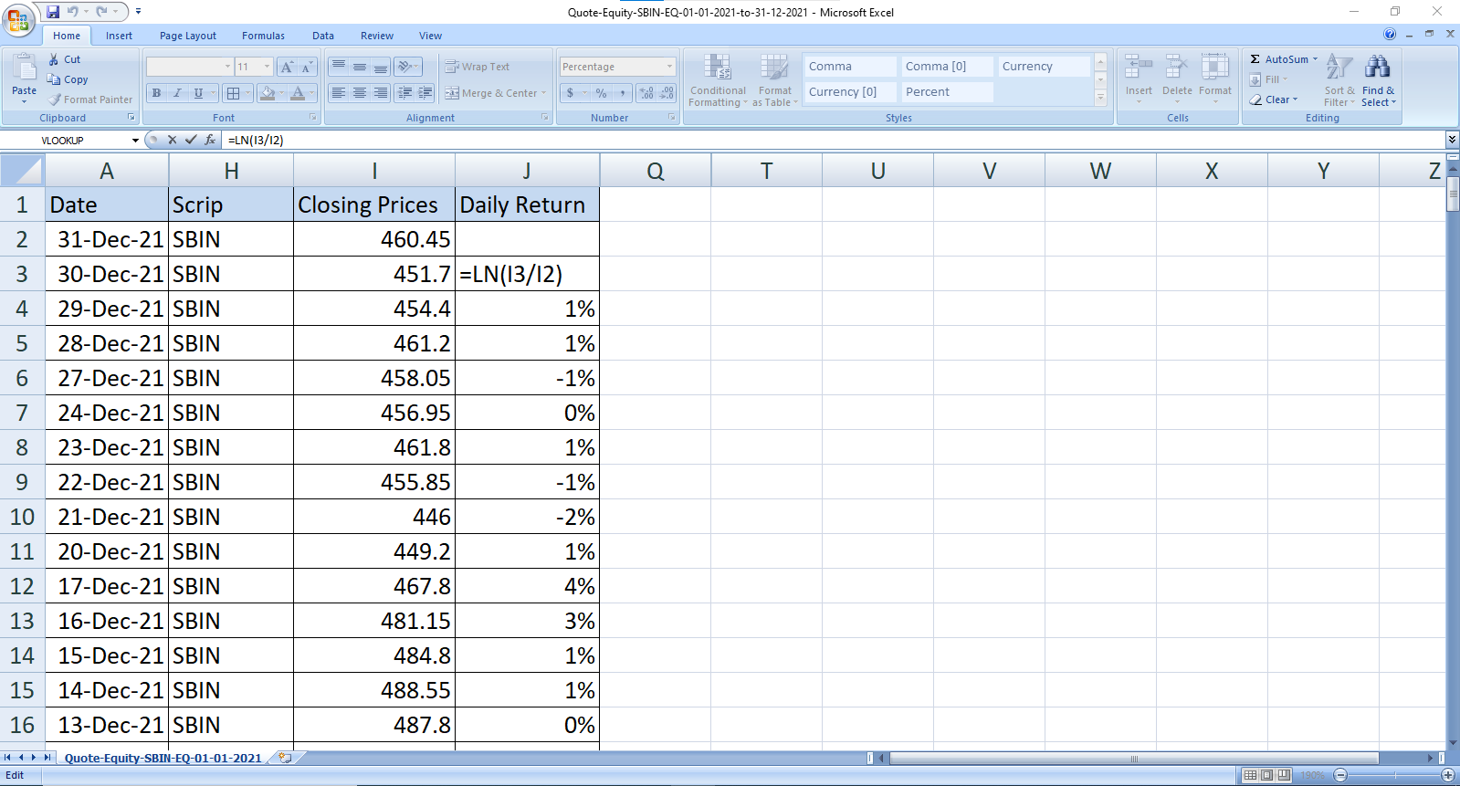
Now using the STDEV function, let me compute the daily volatility:
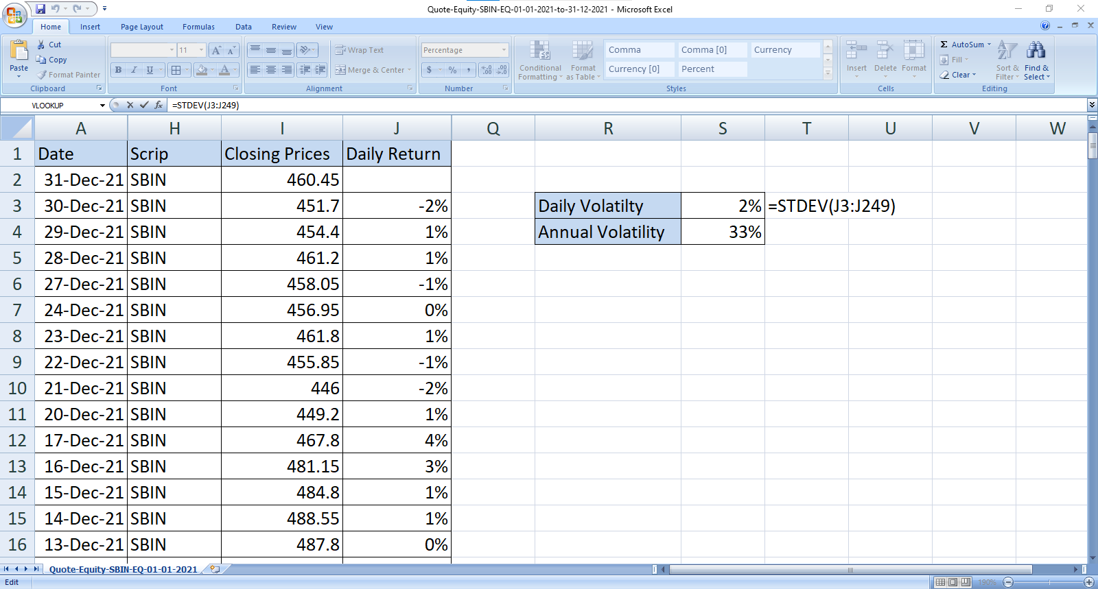
Remember that 3% is the daily volatility that we have computed. To get the annual volatility, we have to multiply it with the square root of time (SQRT is the function that can be used to find the square root of a number).
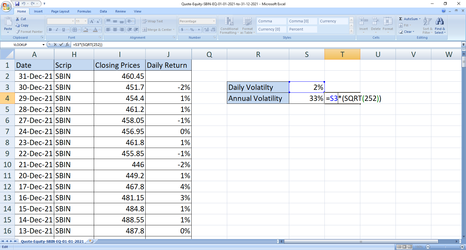
Daily volatility = 2%
Annual volatility = 3% * SQRT(252) = 33%
Likewise, if we have annualized volatility of a stock, we can divide it by square root of time to get the daily volatility.
Volatility And Normal Distribution
We have learnt how to calculate the upper and lower range of a Nifty or a stock by calculating volatility for the same. But how sure are we about this range? There can be chances that Nifty trades beyond this calculated range. Let’s now figure out these chances and also the new range that Nifty trades in.

What we see here is a Galton board, where if we drop small balls from the top, it randomly makes way through the pins and gets accumulated in the panels below. We can notice:
- Most of the balls tend to fall in the central bin.
- As we move further away from the central bin (either left or right) there are fewer balls.
- The bins at extreme ends have very few balls
This kind of distribution is called ‘Normal Distribution’ (the bell curve). The normal distribution curve can be fully described by two numbers- the average and standard deviation.
The mean is the central value where maximum values are concentrated.
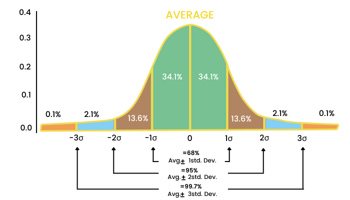
Keeping the average in mind, the data is spread out on either side of this average value. The way the data is spread out is expressed as standard deviation. 1 SD will consider the area shaded in green.
2 SD will consider the area shaded brown and green together on either side.
3 SD will further include the blue area from both the sides.
Now,
- Within the 1 SD we can see 68% of the data.
- Within the 2 SD we can see 95% of the data
- Within the 3 SD we can find 99.7% of the data
If I drop a ball, can you guess which bin it will fall into? I guess not because the ball will take a random walk. However, you can predict the range in which it may fall.
So what will be the range? It can be within 1st SD or the green region in the above chart.
How sure are you about it falling within that range? The answer is 68%
Can we estimate a better accuracy?
Yes. We can increase the range to 2 SD (both the green and brown area) and we can be 95% sure about it.
For even better accuracy of 99.5%, I can say that the ball will fall anywhere within the two blue areas.
So is there no chance for the ball falling in the red region on either side? There is, as low as spotting Black Swan in a river, the probability of the same being as low as 0.5%.
Amazing Fact: At extreme temperatures, Celcius and Fahrenheit tend to be equal. They are the same at -40 C and -40 F. Similarly, at extreme volatility, everything becomes Delta 1.
Types Of Volatility
Volatility measures the magnitude of the change in prices in a security. In an options trade, both sides of the transaction make a bet on the volatility of the underlying security. There are a number of ways to measure volatility, but the two most useful ones are:
- Historical Volatility (HV).
- Implied volatility (IV).
Historical volatility uses the historical data of the security for the computation of the trading range while Implied Volatility accounts for expectations for the future volatility.
Historical Volatility
It gauges the fluctuations of a stock by measuring changes in price over a stipulated period of time. It is less prevalent than IV because it doesn’t give a sneak peek into the future.
When there is a rise in HV, a security’s price will also move more than normal. At this time, traders expect that something will change or has changed. If the HV on the other hand is dropping, it means any uncertainty has been eliminated, so things may run as smooth as they were. Because HV measures past data, traders tend to combine the data with IV at the time of trades.
Implied Volatility
Implied Volatility (IV) is simply an estimate of the future volatility of a stock based on options prices. It gives traders a way to comprehend just how volatile the market will be in the near future. Investors and traders can use IV to price option contracts. Options premium are directly correlated to the volatility expectations. When volatility is expected to be high in future, the option premium will be relatively expensive, whereas if in future, a lower volatility is expected, an option will have relatively low premium.
IV generally increases when there is an event or announcement coming up, and it has a tendency to decrease after that announcement or event has passed. So you may want to factor this in analyzing an option’s IV, especially for options that are close to expiry.
When IV is significantly higher than the average historical levels, options premium are assumed to be overvalued. These options are advantageous to option sellers. In such situations, the objective is to square off positions and pocket profit as volatility slides down to average levels and the option premium declines. Option buyers on the other hand, have an advantage when the IV is significantly lower than the HV, indicating undervalued options premium.
The VIX Index
Now that we have understood the concept of volatility and its types, next in this chapter, we will learn how to track the volatility with the help of ‘VIX.’
VIX, or the Volatility Index, is used to measure the near term volatility expectations of the market. The Chicago Board Options Exchange (CBOE) introduced volatility as an asset class in the form of an index in the year 1993. It gained immense popularity after its launch. Hence (CBOE) introduced trading on the VIX derivative in the year 2004.
The volatility index and Market index are completely different. The market index measures the direction of the market, calculated by the price movements of the underlying stocks. However, the volatility index measures the volatility of the market and is calculated using the order book of the underlying index's options. Another difference is that the market index value is expressed in numbers, whereas the volatility index is expressed as an annualized percentage. The volatility index based on the order books of Nifty options is known as India VIX.
IMPORTANCE OF INDIA VIX:
India VIX was launched by the NSE in 2008, followed by NVIX Futures in 2014. India VIX indicates the Indian market's volatility from the investor's point of view. Volatility and the value of India VIX move together or in parallel. A higher value of India VIX indicates higher volatility expectations. This means that a significant change in Nifty and a lower value of India VIX will result in a minimal change or lower volatility expectation.
There is an inverse relation between India VIX and Nifty. The India VIX represents the risk factor in the stock market. Therefore, an increase in India-VIX means an increase in risk. Therefore the market falls. If the India VIX is decreasing, then it means that the market should go up due to the low-risk factor in the market.
Volatility Smile
Earlier, we learned the concept of implied volatility which is an estimate of future volatility. Now in this chapter, we will study a pattern of implied volatility (IV) known as 'Volatility Smile.'
Volatility smiles are IV patterns that develop while pricing options. When the IV of options (with the same expiration date, underlying asset, but different strike prices) is plotted, the graph has a tendency to show a smile.
Changes in volatility for options:
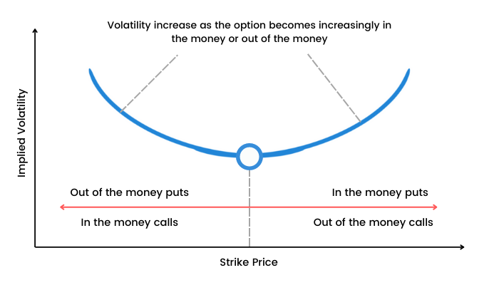
Volatility smile shows the more the option is in ITM or OTM, the greater the IV becomes. IV tends to be lowest for ATM options.
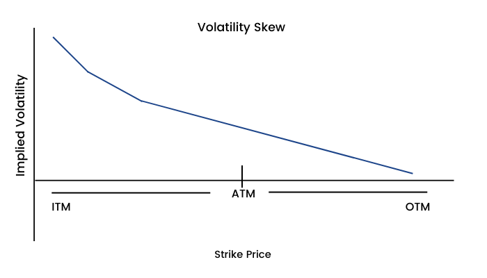
This smile is known as Volatility Skew. It is interesting that this pattern has existed only since the stock market crash of 1987. Prior to October 1987, implied volatilities were not much dependent on strike prices. This led to a conclusion that one reason for the equity volatility skew may be ‘crashophobia’. Since then traders are concerned about the possibility of a similar crash, they price the options accordingly.
'Volatility smile' is generally observed in near term equity options and forex options. However, index options and long term equity options tend to have a volatility skew.
Delta Neutral Hedging
In options trading, the "Greeks" provide valuable understanding of risk associated with a particular option.
Theta tells us how much we are receiving or paying every day, vega tells us how much we can gain or lose because of volatility, and delta tells us how much an option's value will change as the price of the underlying fluctuates.
Delta is a somewhat unique "Greek," because the term may also be used to describe the directional exposure of a position.
For example, if a trader buys a naked long call, this position will have a "long delta" because we gain as the underlying goes up. Here the risk is defined because the trader can lose only the premium he has paid for the call.
The term "delta neutral" refers to a strategic trading approach that attempts to neutralize directional exposure, using the underlying security of the option. In simple terms, trading delta neutral can help traders reduce their exposure if a position moves against them. However, he certainly has to pay a price for risk mitigation, which can be a substantial part of his profit.
Traders use Delta-neutral strategies to profit from either IV or from time decay of the options. Usually, traders purchase securities that are inversely related to their original position. In case of adverse price movement, the inversely related security will move in the opposite direction, acting as a hedge against the losses. Let’s take an example to understand it better.
Imagine that two different traders decide to invest in a certain stock, say XYZ Ltd. which is currently trading at ₹200 per share, and the company is set to report earnings in two weeks.
Intending to profit on a quick rise in the stock price after a good earnings report, both traders decide to purchase 200 options of the 220 strike calls that expire in three weeks. They each pay ₹5 for the 220 strike calls, which equates to an outflow of ₹(5*200) = ₹1000.
Suppose, Trader A decides to sit tight with the naked calls while Trader B decides to hedge himself and create a delta neutral position. This means that Trader B will use the underlying stock to “neutralize” the long delta exposure of the calls.
Trader A: Trader A purchases 200 of the 220 strike calls for ₹5. Trader A does not take any position in stock against the long calls.
Trader B: Trader B purchases 200 of the 220 strike calls for ₹5. The 220 strike calls have an associated delta of .35, and Trader B decides to hedge the position "delta neutral." This means Trader B sells 70 shares of stock XYZ short against his call position.
Now let's look at some hypothetical situations for the day of earnings, and see how each of the respective traders (A and B) perform :
Scenario #1: Company XYZ reports fantastic earnings and the stock opens trading ₹240 after earnings are released.
- Trader A: Trader A paid ₹5 for 200 calls that are now worth ₹20. Trader A makes a profit of ₹3,000 on the trade (15 x 200).
- Trader B: Trader B also paid ₹5 for 200 calls that are now worth ₹20. However, Trader B additionally sold 70 shares of stock XYZ short for ₹200/share. That means Trader B has made ₹3,000 on his call position, but lost ₹40/share on the short shares (40*70 = 2,800). Trader B, therefore, makes a profit of ₹200 on the trade (3000-2800).
Scenario #2: Company XYZ reports fantastic earnings, but simultaneously announces accounting irregularities at the firm that are currently being investigated. Stock XYZ opens at ₹180/share after earnings are released.
- Trader A: Trader A paid ₹5 for 200 calls that are now worth nothing, very likely will expire worthless. Trader A will likely lose his entire ₹1,000 investment in the call premium.
- Trader B: Trader B also paid ₹5 for 200 calls that are now likely to expire worthless too. Trader B will likely lose his entire ₹1,000 investment in the call premium. However, Trader B also sold 70 shares of stock XYZ short for ₹200/share. That means Trader B has made a profit of ₹20/share on the short shares (20*70=1400). Trader B therefore makes a profit of ₹400 on the trade (1400-1000).
This shows how a delta-neutral trading approach affects profit and loss for a position.
Traders can use this framework to ensure they have deployed a position that matches their outlook, expectations, and risk profile.
Any position, no matter how complex, is simply the sum of its parts. By breaking down the P/L of each component of a trade, traders can best understand how different moves in an underlying will affect the overall position, and more importantly, the bottom line.
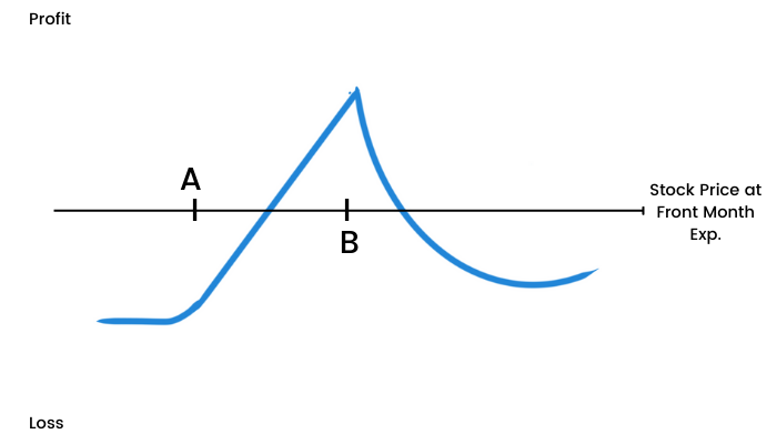
Calendar Spread
In this chapter, we will learn an option trading strategy called ‘Calendar Spread.’
As the name suggests, it spreads over the calendar month, hence is known as Calendar spread. The logic behind calendar spread is that near month options price fluctuate more than far month.
Calendar spread can be of many types. If it is made using the call option it is called Calendar Call Spread, similarly for put it is known Calendar Put Spread.
If the Calendar Spread is made of a different month’s expiry but same strike price, it is called Horizontal Spread.
If it is made using same month expiry options but different strike price, it is called Vertical Spread. Lastly, when both the strike prices and expiry months are different, it is called Diagonal Spread.
Here, the aim is to lock in profits from changes in volatility over a period of time. One can exploit fluctuation in pricing from short-term events.
Typically, long calendar spread involves buying a far-term option and selling a near-term option that is of the same type and exercise price. A calendar spread is most profitable when the underlying asset does not move significantly in either direction until after the near-month option expires. The two identical contracts create a difference in price because of time value -specifically the amount of time that differs between the two contracts.
The goal of a calendar spread strategy is to take advantage of differences in volatility and time decay, while also trying to minimize the impact of movements in the underlying security. Depending on where the stock is relative to the strike price when implemented the forecast can either be neutral, bullish or bearish.
The long trade takes advantage of how near- and long-dated options act with change in time and volatility. An increase in IV would have a positive impact on this strategy because longer-term options are more sensitive to changes in volatility (higher vega). The caveat is that both the options may trade at different IV, but it rarely happens that the movement of volatility and the effect on the price of the spread is different from expectation.
Since this spread involves premium outflow, the maximum loss is the amount paid for the execution of the strategy. The option sold is closer to expiration and therefore has a lower price than the option bought, resulting in a premium outflow.
Ideally, we will want the market to be steady or decline slightly during the near term expiry and thereafter move higher strongly during the long term expiry. We also expect a sharp increase in IV during the long term expiry.
At the expiration of the near-term option, the maximum gain would occur when the underlying asset is at or slightly below the strike price of the expiring option. If the asset were higher, the expiring option would have intrinsic value. Once the near-term option expires worthless, the trader is left with a simple long call position, which does not cap profits on the higher side.
Basically, a trader with a bullish longer-term view can reduce the cost of purchasing a longer-term call option and selling the shorter term call option.
Let’s consider an example:
With Nifty trading at 17200 in January:
- Sell the January 17300 CE @ 200/-
- Buy the February 17300 CE @ 420/-
Net cost comes to (420-200)= 220/-
Since this is a debit spread, the maximum loss is the amount paid for the strategy. The option sold is closer to expiration and therefore has a lower price than the option bought, yielding a net debit or cost. In this scenario, the trader is hoping to capture an increase of value associated with a rising price (up to but not beyond 17300) by January expiration.
The ideal market move for profit would be for the price to become more volatile in the near term, but to generally rise, closing just below 17300 as of the January expiration. This allows the January option contract to expire worthless, and still allow the trader to profit from upward moves up until the February expiration.
If the trader was to simply buy the February expiration, the cost would have been ₹420, but by employing this spread, the cost required to make and hold this trade was only ₹220, making the trade one of greater margin and less risk.
Depending on which strike price and contract type are chosen, the strategy can be used to profit from a neutral, bullish or bearish market trend.
Diagonal Spread With Calls
The next strategy that we will study is called “Diagonal Spread.” It can be either created by Call options or Put options.
First, let us understand with calls:
You can think of this as a two-step strategy. It’s a cross between a long calendar spread with calls and a short call spread. It is a time decay play. Ideally, you will be able to establish this strategy for a net credit or for a small net debit.
I’m using the example of one-month diagonal spread. But please note, it is possible to use different time intervals. If you’re going to use more than a one-month interval between the near-month and far-month options, you need to understand the ins and outs of rolling an option position.
This spread involves selling an OTM call (say at strike 17500 when Nifty is trading at 17300) for the near month expiry (e.g. January) and buying a further OTM call (say for strike 17700) of the next month expiry (say February). At expiration of the January call, one shall again sell another call for strike 17500 but now for February expiry.
This strategy is to be executed when you are expecting neutral activity in the near term expiry month, and neutral to bearish activity during the next month.
Maximum profit is limited to the net premium received for selling both calls of strike 17500, minus the premium paid for the call of strike 17700. For step one, you want the Nifty to stay at or around 17500 until January expiry. For step two, you’ll want the Nifty to be below 17500 during February expiry.
Because there are two expiration dates for the options in a diagonal spread, a pricing model must be used to guess and estimate what the value of the far-month call will be when the near-month call expires.
The risk in this strategy is the difference between both the strikes, that is 200 – difference between 17700 & 17500 (of course we have to adjust the net premium inflow/outflow accordingly).
For this strategy, before January expiration, time decay is your friend, since the shorter-term call will lose time value faster than the longer-term call. After closing the January call with strike 17500 and selling another call of the same strike but February expiry, time decay is somewhat neutral. That’s because you’ll see erosion in the value of both the option you sold (good) and the option you bought (bad).
After the strategy is established, although you want neutral movement on Nifty if it’s at or below 17500, you’re better off if IV increases close to near-month expiration. That way, you will receive a higher premium for selling another call at 17500.
After January expiration, you have legged into a short call spread. If the forecast you made was correct and Nifty is approaching or below 17500, you want IV to decrease. That’s because it will decrease the value of both the options. Preferably you want them to expire worthless.
But if your forecast was incorrect and Nifty is approaching or above 17700, you want IV to increase. Firstly because it will increase the value of the option you bought faster than the option you sold, thereby decreasing the overall value of the spread. Secondly because it shows a higher probability of a price swing (hopefully a decline).
Ideally, you want some initial volatility with some predictability. Some volatility is good, because the plan is to sell two options, and you want to get as much as possible for them. On the other hand, we want the stock price to remain stable. That’s a bit of a paradox, and that’s why this strategy is for more advanced traders.
To run this strategy, you need to know how to manage the risk of early assignment on your short options.

Diagonal Spread With Puts
Again, let us discuss 'Diagonal Spread' now using Put options.
This again is a two-step strategy, which is a cross between a long calendar spread with puts and a short put spread. Here again we can play with different maturities.
This strategy involves selling an OTM put (say for strike 17500 for January expiry when Nifty is trading at 17600) and buying a further OTM put (say strike 17300 for February expiry). When the January put expires, we sell another put of strike 17500 (but now for February expiry).
Here, we expect neutral activity in the month of January, then neutral to bullish activity during the month of February.
For this strategy, before January expiration, time decay is our friend, since the shorter-term put will lose time value faster than the longer-term put. After closing the January put of 17500 and selling another put with the same strike but with February expiry, time decay is somewhat neutral. That’s because we’ll see erosion in the value of both the option we have sold (good) and the option we bought (bad).
After the strategy is established, although we want neutral movement on Nifty, we’re better off if IV increases close to January expiration. That way, we will receive a higher premium for selling another put at 17500.
After January expiration, we have legged into a short put spread.
If our forecast was correct and Nifty is approaching or above 17500, we want IV to decrease. That’s because it will decrease the value of both the options. Again here we want them to expire worthless.
If our forecast was incorrect and Nifty is approaching or below 17300, we want IV to increase. Firstly because it will increase the value of the near-the-money option we bought faster than the in-the-money option we sold, thereby decreasing the overall value of the spread. Secondly because it shows a higher probability of a price swing (hopefully be to the upside).
Gamma Delta Neutral Option Strategy
By now, we very well know that by hedging the net gamma and net delta of our position, we can safely keep our position direction neutral. Traders use this strategy to minimize their exposure to volatility. It is also a very good strategy to secure the profits generated by a trade so far.
We will use a ratio call write (A ratio call write is an option strategy similar to a covered call, where an investor owns shares in the underlying stock and then writes/sells more call options than the shares owned. The objective of a ratio call write is to capture the additional premiums received by selling the option. We will buy options at a lower strike price than that at which they are sold.
For example, if we buy the Nifty call option with a 17000 strike price, we will sell the call option at a 17500 strike price. We will adjust the ratio of buying and selling options to eliminate the net gamma of our position.
We know that in a ratio write options strategy, more options are sold than purchased. This means that some options are sold "naked” which can prove to be very risky. The risk here is that if the stock rallies enough, we will lose money because of the risk involved by selling naked options. By reducing the net gamma to a value close to zero, we eliminate the risk of delta changing significantly (assuming a very short time frame).
To effectively neutralize the gamma, we first have to find the ratio at which we will buy and sell. We can quickly find out the gamma neutral ratio by doing the following:
- Find the gamma of each option.
For example, if we have our Nifty 17000 call with a gamma of 0.0007 and our 17500 call with a gamma of 0.0005, we would buy 5 contracts of 14000 calls and sell 7 contracts of 17500 calls. Remember this is per share, and each option represents 50 shares.
- Buying calls with gamma of 0.0007 is a gamma of (50*5*0.0007) =0.175
- Selling calls with gamma of 0.0005 is a gamma of -(50*7*0.0005)=-0.175 (Negative because we are going short on options)
This adds up to a net gamma of 0. Because the gamma is usually expressed in up to three decimal places, your actual net gamma might vary by very points from zero. After the gamma is neutralized, we will have to make the net delta of our position to zero. If our 17000 calls have a delta of 0.56 and our 17500 calls have a delta of 0.23, we can calculate the following.
- 5 contracts of 17000 call bought gives us a delta of (0.56*5*50)= 140
- 7 contracts of 14500 call sold gives us a delta of (-0.23*7*75)= -80.5
This results in a net delta of positive 59.5. To make this net delta very close to zero, we can short 59 shares of the underlying stock. This is because each share of stock has a delta of 1. This adds -59 to the delta, making it -0.25, very close to zero. Because you cannot short parts of a share, -0.25 is as close as we can get the net delta to zero.
Now that our position is effectively price neutral, let us compute its profitability. The 17000 calls have a theta of -5.5 and the 17500 calls have a theta of -4.1. This means:
- 5 contracts of 17000 call bought gives us a theta of (-5.5*5*50)= - 1375
- 7 contracts of 17500 call sold gives us a theta of (4.1*7*50)= 1435 (positive because we are selling options)
This results in a net theta of 60. This can be interpreted as your position making ₹60 per day. You'll have to hold your position because option behavior is not adjusted daily.
A few risks are associated with this strategy. Very large price moves can throw this out of proportion. If we hold the position for a week, adjustment of ratio and delta hedge is not required. However, if held for a longer time, the stock price will have more time to move in one direction.
The position's value can change dramatically because of changes in IV, because volatility is not hedged here. Although the risk of daily price movement has been eliminated, we have another risk factor to worry about, i.e. increased exposure to changes in IV. Changes in volatility have a small role to play in your position over a short time period of a week.
The risk of ratio can be minimized by adjusting positions in the underlying stock and also by hedging certain characteristics of the options. By doing this, we can profit from the time value of the options sold.
Gamma Scalping Strategy
Scalping a unique trading style where a trader tries to make a small profit by buying and selling considerable securities in a short time frame. Now, in this section, we will learn an option trading strategy using one of the option-greeks called ‘Gamma Scalping.’ So, let us begin:
As stock prices in a portfolio keep fluctuating, it requires adjustments in order to keep its delta neutral. For example, if a trader buys call option, he will go short on stock to hedge his position. But when it comes to large portfolios which follow a delta neutral approach, occasional adjustments will be required to keep it delta neutral.
A very systematic approach to these adjustments is "gamma scalping" or "gamma hedging." Gamma scalping is not an individual strategy - rather, it is layered upon a volatility strategy.
There are traders who use "scalping" as a standalone strategy just to make small profits with price fluctuations. However, scalping gamma is different. It is hooked around delta adjustments in an option portfolio.
Imagine a large portfolio that consists of both long and short premium positions. Long premium positions will want the underlying to move a bit, while short premium positions will want the underlying to be stable.
In other words, the risk involved with the long premium position is lack of movement, while the risk involved with the short premium position is significant movement in the wrong direction. These risks can be reduced with the help of gamma adjustment strategy.
A long premium position is the basis of true gamma scalping. Due to the positive relationship between underlying price and delta, your position delta will decrease when the underlying moves against you and increase when the underlying moves for you. As this happens, you “gamma scalp” your position by adding stock position whether long/short to bring the overall delta back to zero. The objective here is to neutralize the cost of theta on the long premium position. Elections, earnings, economic data etc are all good reasons to think that the market can give a potential move and the exact time to initiate a true gamma scalp strategy.
Master Options Scalping: Elevate Your Trading Skills Now!
Let us take an example of a long straddle:
Gamma Scalp Setup:
- Buy a Straddle (Long Call + Long Put)
- Perfectly Data Neutral
If the underlying falls: Add a long stock
If the underlying rises: Add a short stock
We start by buying a straddle (call and put option of the same strike price), expecting the market to either go up or go down. So to start off, I have a delta neutral position. When the market goes down, according to gamma scalping, my delta is now approaching a higher negative value because of the put. The negative delta of Put is going to overshadow the delta of long calls. To restore to a delta neutral position, I will add stocks to add delta and thus making delta neutral again. Similarly when the underlying rises, the call delta increases and the entire delta of my position heads to become a positive value. Thus, to restore my delta neutrality, I will now sell the stocks to get a negative delta. It will again help me re-establish a delta neutral position. The reason behind this continuous adding and selling of stock to maintain delta neutral position is theta. We are long on straddle and theta is acting against us every single day. If the price of the underlying doesn’t move, we will lose time value on both the long options.
Imagine a trader has bought 100 lots of Nifty 17000 CE when Nifty is trading at 16000. The premium for this call is ₹60. Delta of this option should be close to 0.25. The delta of the position is (0.25*100)= 25
In order to be delta neutral, he will sell 25 lots of Nifty. If Nifty rises to 16500, the delta of this call option will range approximately at 0.4. So now the total delta of the option position is (100*.4) = 40 which means he will have to sell 40 lots of Nifty. He has already sold 25 lots, so now he has to sell the remaining 15 lots at the price of 16500.
Selling these 15 lots is gamma scalping in action. This adjustment makes the portfolio delta neutral and also gives a chance to profit if Nifty again lowers to 16000. This back and forth adjustment or scalping produces extra income to help cover the cost of theta.
There is no fixed solution as to when these adjustments should be made because it depends on the risk profile and adjustment strategy of an individual.
Let us consider a situation when Nifty is trading at 16500. You buy 100 lots of straddles at a strike price 16500. The 16500 CE is trading at ₹370, whereas the 16500 PE was trading at ₹400. So the total straddle value that you pay is (370+400) = ₹770
So the breakeven points for you are (16500-770)= 15730 and (16500+770) = 17270
Combined Theta for this position comes to -10.75 (as derived from the Black–Scholes model option pricing calculator). This means that this entire position is going to cost you ₹10.75 daily as the premium erodes while you wait for Nifty to make some move.
Say, after four days, Nifty bounces up to 17000 level. So now the price of the call is ₹640 whereas the price of the put is ₹185. This brings the straddle value to (640+185) = ₹825
So clearly we gain on straddle because we bought it at ₹770/- and now it’s worth ₹825/-.
Now the position delta here is, call delta= 0.7 and put delta=-.3 which comes to a delta of 0.4. Trader had bought 100 lots, so his delta is 0.4*100 = 40
To gamma scalp and establish a delta neutral position he will sell 40 lots of Nifty.
Now let us assume after seven more days have passed and Nifty is again trading at 16200 level. Now the straddle value will be (210+440)= ₹650/- (call premium now becomes 210 and put premium 440).
Now we lose on straddle which was bought at 770 and now trades at 650. But we gain on Nifty because we sold it for 17000 and it now trades at 16200. So profit on Nifty is 800*40 lots = 32000/-
Delta of the position now: call delta =0.4 put delta = -0.6. So net delta = -0.2*100=-20
To neutralize this position we will buy 60 lots of Nifty. (40 to square off and 20 to neutralize delta).
As four more days pass and Nifty slides further to 16000. Now the straddle value comes to (120+560)= 680. We still lose on the straddle. We lose on Nifty (20*-200)= -4000 but we gained 32000 from the previous Nifty trade.
So here we see when the Nifty does not move much we tend to suffer losses. The best case scenario for us will be the underlying to explode in either direction, when buying a straddle. Another scenario suitable for us will be heavy continuous price swings. This is so because it helps add short delta at the top and positive delta at the bottom. This process of buying low and selling high, obviously helps to make more money and effectively the long straddle becomes free. Now, we have no fear of losing premium money.
Another scenario is where the underlying barely moves and doesn’t give the opportunity to scalp gamma.
Reverse gamma scalping is very much the opposite. Here you start with a short premium position, like a short straddle. You scalp the short-term price swings in the underlying, but in a completely different method. Instead of buying when the price falls and selling when the price rises, you actually buy when the price rises and sell when the price falls. This is because the short gamma with the short premium position makes you bearish on the way up and bullish on the way down. Therefore, you continue to work to neutralize your delta, and you’re willing to give up some of your positive theta in exchange for some risk reduction on your naked options.
In both the cases, the objective was to scalp around the original position. The two reasons why we scalp? The answer is to neutralize delta and adjust theta.
Put Call Parity
Before we move on to further option trading strategies, we need to learn an important concept called ‘Put-Call Parity.’
The put-call parity helps you to understand the impact of demand and supply on the option price, and how option values are inter linked across different strikes and expirations, given that they belong to the same underlying security.
The term ‘parity’ refers to the state of being equal or having equal value. Options theory is structured in such an ingenious fashion that the calls and puts complement each other with regards to their price and value.
So, if you are aware of the value of a call option, you can easily calculate the value of the complimentary put option (which has the same expiration date and strike price). This knowledge is very essential for traders. Firstly because it can help you figure out profitable opportunities when the option premiums are not functional. A thorough understanding of put-call parity is also important because it helps you to work out the relative value of an option you are considering to add to your portfolio.
Suppose a trader holds a short put (European) and a long call (European) of the same class. According to the Put-call parity, this is equivalent to having one future contract of the same asset and same date of expiry, and future price that is the same as the strike price of the option.
In situations when the put price diverges from the call price, an arbitrage opportunity comes into existence. This means that traders can make a profit without taking any risk. However, as mentioned earlier, even in liquid markets, chances of this sort are a bit uncommon and have a small window.
Put Call Parity is stated using this equation:
Call + Strike = Put + Futures
Here,
Call means the price of the call option,
Put means the price of the put option,
Futures means the future price and
Strike means the price for which call and put are considered.
Having clarified that, let us understand how it works with the help of an example. Suppose Nifty is trading at 16940. So the ATM option will be 17000. You buy a call option and sell a put option of the same strike. The date of expiration is a month from the date of purchase. The call option costs ₹35 and the put option costs ₹90. So, the net inflow is (90-35) = ₹55/-
Let us consider a few scenarios to understand the trade better.
Nifty expires 16000 (below ATM):
Here the 17000 CE expires worthless because it is now OTM. Hence, we lose ₹35 which we had paid as its premium. For, put option, we suffered losses because we had sold the put option (bullish position) and the market went in the opposite direction on the downside. So, the loss here = (16000-17000 +90) = - ₹910/-
Nifty expires at 17000 (ATM):
In this case both the options expire worthless again. So we lose the premium paid for call and retain the premium received for put. So the difference of both the premium stays with us, i.e. ₹55/-
Nifty expires at 18000 (above ATM):
Here the call options start paying off because of the bullish position. So profit on call option = (18000-17000-35)= ₹965/-
The put option expires worthless because of being OTM. So we retain the premium of ₹90 from the put as well.
Hence, the total profit in this scenario = 965+90 = ₹1055/-
If you construct a graph by plotting the profit or loss one has on these positions for different prices of Nifty, some interesting things will come to light.
Suppose the long call’s profit/loss is combined with the short put’s profit/loss. We will make a profit or loss of the exact amount we would have if we just took a future contract of Nifty at 17000, which has a validity of one month. If Nifty trades lower than 17000, you will incur a loss. If it trades higher, you will make a profit.
Here, we are not taking transaction fees into consideration.
To understand the put-call parity better, you can also compare the performance of a fiduciary call and a protective put of the same class. Protective put is a combination of a long stock and a long put position. This limits the negative impact of holding the stock. A fiduciary call is the combination of a long call and stock which is equivalent to the strike price’s present value. This ensures that the investor gains enough money to make use of the option on its expiry.
Talking about the equation again,
Call + Strike = Put + Futures
In situations where one side of this equation is heavier than the other, this is when an arbitrage opportunity is present. A hassle-free profit is locked in when a trader sells the expensive side of the equation and buys the cheaper side. In real life, however, the occasions where one can take advantage of arbitrage are hard to come across and short-lived. Also, sometimes the margins offered by these are so tiny that you will need to invest a huge capital to use it advantageously.
Options Arbitrage
In this chapter, we will learn ‘Options Arbitrage’. But what exactly is arbitrage?
Arbitrage is the opportunity to make risk-free profit by simultaneously buying an underpriced asset and selling it at market price.
Options arbitrage is the use of options to reap marginal risk-free profit by locking value created through violation of Put-Call Parity.
The only drawback of options arbitrage is that profitable opportunities are hard to come by and gets filled out extremely fast by computers and system trading used by financial institutions which monitor for such opportunities all the time.
An inequality in price of the security must exist for arbitrage to work. When a security is underpriced in another market, you simply buy the underpriced security in that market and then sell it at the market price in this market simultaneously to reap a risk free profit. A call option can be underpriced compared to other options of the same expiry or same options with different expiry. All these are governed by the principle of Put Call Parity. When this principle of Put Call Parity is violated, opportunities of options arbitrage comes into the picture.
Conversion-Reversal Arbitrage
After learning Options Arbitrage, here we will understand the ‘Conversion Reversal Arbitrage.’
Conversion and reversal arbitrage is a strategy which takes advantage of differences in the value of synthetic positions and their equal in order to return a risk free profit.
Conversion arbitrage is an options trading strategy to exploit inefficiencies that exist in option pricing. Conversion arbitrage is a risk-neutral strategy, where a trader buys a put and writes a covered call (on a stock that the trader already owns) with the same strike prices and expiration dates.
A trader will profit from a conversion strategy when the call option is overpriced or the put option is underpriced. This can be due to market inefficiencies, or from the effects of mispriced interest rate assumptions.
Conversion arbitrage is a strategy which can be carried out for riskless profit when options are either overpriced or underpriced.
Let me just mention how a synthetic position is created. There are six basic synthetic positions relating to combinations of put options, call options and their underlying stock:
- Synthetic Long Stock = Long Call + Short Put
- Synthetic Short Stock = Short Call + Long Put
- Synthetic Long Call = Long Stock + Long Put
- Synthetic Short Call = Short Stock + Short Put
- Synthetic Short Put = Short Call + Long Stock
- Synthetic Long Put =Long Call + Short Stock
In order for the synthetic trades to work, all options used together must be of the same expiration, strike and underlying.
Synthetic position allows an open option position to be synthetically squared off without selling the position itself. For example, a synthetic long stock can be squared off by shorting an equivalent amount of the actual stock. Synthetically closed positions are not subject to directional risk and hedges against short term price movement.
In simple words, a Conversion is when stock is being bought in order to synthetically close out a short stock position that is created synthetically by long put and short call of the same strike. Reversal is when stock is being shorted/ sold in order to synthetically close out a synthetic long stock position. However, conversion and reversal do not necessarily apply only to synthetic long and short stocks.
In fact, whenever a synthetically closed position involves a long stock, it is known as a Conversion and whenever it involves a short stock, it is known as a Reversal. For example, a synthetic call option (a long put and a long stock) can be synthetically squared off by shorting a call option. This is known as a conversion, as the entire position involves a long stock. A synthetic put option (a long call and short stock) can be synthetically squared off by shorting a put option. This is known as a reversal as it involves a short stock.

There are important risk factors to keep in mind for arbitrage conversions, like a hike in interest rates and the elimination of dividends.
When a position is synthetically closed, it is exposed only to theta risk, which is time decay. When put-call parity is in force perfectly, the extrinsic value of the synthetic position should be just the same as the extrinsic value of the actual instrument.
For example, a synthetic long stock should have no extrinsic value at all as the premium of the put option cancels out the premium of the call option involved. A synthetic long call should have the same extrinsic value as the actual call option itself. However, there are conditions when 'Put Call Parity' is severely violated that a significant difference in extrinsic value exists between a synthetic position and its actual instrument. When such a position is synthetically closed out, it results in profit from that difference in extrinsic value on expiry. This is known as Conversion/Reversal Arbitrage.
Traders use conversions when options are relatively overpriced and use reversals when options are relatively underpriced. Conversion and Reversal can also be carried out between options and futures instead of the underlying stock. A well executed Conversion and Reversal Arbitrage has no chance of loss, irrespective of how the underlying moves.
Box Spread
The last strategy that we will learn is a ‘Box Spread.’
The Box Spread is a complex four legged options trading strategy designed to take advantage of differences in options prices for a risk-free arbitrage.
Such situations occur when the Put Call Parity is violated by strong, short term shift in demand in the options market. When such a situation occurs, a Box spread can be used to "box in" the profit because of the imbalance.
However, such discrepancies are so short-lived and marginal that it is hard to execute a Box Spread fast enough. Box spreads should be used when one detects a violation of Put Call Parity. Put Call Parity is violated all the time in the market. But most of these violations are so insignificant that an arbitrage opportunity does not exist when commissions are involved. There are many ways to test for a significant violation of Put Call Parity and such profitable opportunities are so rare and tend to fill out so quickly that softwares are used to detect and execute the spread.
Box spreads open up an arbitrage opportunity without the use of the underlying itself. There are two types of Box spreads:
- Long Box Spread
- Short Box Spread
A long box spread includes buying a bull call spread with a matching bear put spread. These vertical spreads must have the same strike prices and expiration dates.
So a Box Spread consists of 4 options across 2 strike prices. They are:
Buy ITM Call + Sell OTM Call + Buy ITM Put + Sell OTM Put
Strike price of the ITM call and OTM put must be the same. Similarly, strike price for the OTM Call and ITM put must be the same. This results in a position that looks like the table below:

X1 = In The Money Strike Price
X2 = Out Of The Money Strike Price
The above table clearly shows that the Box Spread is a combination of a Bull call spread and a Bear put spread across the same strike prices. Another way of understanding box spread is that it is actually a combination of a Synthetic Long Stock and a Synthetic Short Stock.
A bullish vertical spread maximizes its profit when the underlying closes at the higher strike price at maturity. The bearish vertical spread maximizes its profit when the underlying closes at the lower strike price at maturity. By combining both the bull call spread and the bear put spread, a trader removes the risk of the price of underlying at the expiry. This is so because the payoff is always the difference between the two strike prices at the time of expiry.
If the cost of the spread is less than the difference between both the strike prices, then the trader has locked in a risk-free profit also making it a delta-neutral strategy. Otherwise, the trader has incurred a loss which is the cost to execute this strategy.
- Box value (at expiration) = Higher strike price – Lower strike price
- Maximum Profit = Box Value – Net premium paid
- Maximum loss = Net premium paid
Once the Box Spread is executed, you will have to wait till expiration and then close the position for the profit pocketed. A short box spread can be used when the net debit is higher than the expiration value. A Short Box Spread is just reversing the buys and sells of a long box spread.

Conclusion
Finally, now at the end of this module, we have learned that the price of an option largely varies for five factors: Delta, Gamma, Vega, Theta and Rho. These are combinedly known as Option Greeks. Not only that, we have learned how these options greeks affect the change in the price of an option but also discuss why they affect. For a trader, it becomes easy to trade options when they are completely aware of how and when the different options greeks affect the price at different time periods.
A 360 degree knowledge of options greeks helps a trader to implement several options strategies in the best possible manner that eventually increases the profitability while trading in the market. It is now time for you to implement these strategies you have learned from this module but don't expect a quick and huge chunk of money easily. This is because expertise comes with time and effort. So, keep practicing and develop your trading skills.


