Introduction to Financial Modeling

A lot of people, years into their marriage, often wonder whether there could have been an effective mechanism to forecast the success of the relationship – an Excel tool where one could plug into variables related to the bride and the groom – and the model would come up with a prediction – “Hey, there is an 82% probability that you will make a great couple”

Unfortunately, such a tool doesn’t exist and we have to brace ourselves to live with our spouses as they are 

However, we are lucky that when it comes to making decisions like the ones related to intrinsic value, valuations, mergers & acquisitions, project financing etc., we have the financial model come to our rescue. 

A financial model is simply a tool that’s built in, say, MS Excel to forecast a business’ financial performance.  The forecast is typically based on the company’s historical performance, assumptions about the future, and requires preparing an income statement, balance sheet and cash flow statement. 

The corporate world is struggling to find enough professionals who can prepare financial models for complex business models and yet make them SIMPLE TO UNDERSTAND. The intellect and interest lies in making a simple, scalable and robust model.

Concept

So let’s say, you have a power plant as follows on the left side of the image but you can also build a working model of the power plant like you see on the right side of the image:

So, a model is a representation, generally in miniature, to show the construction or appearance of something.

Remember that financial models apply not only to a company but also to personal finance. We will discuss both of them in the subsequent units.

Building a Personal Financial Model

Let us start with preparing a financial model based on personal finance.

Personal Finance is all about handling and managing your own money – be it income, expenses, savings, investments, insurance, etc. A Financial Model can help an individual to analyse his personal financial situation by representing it in a spreadsheet.

The four important pillars of a personal finance model are –

• How much money comes in?
• How much money goes out?
• What do you own?
• What do you owe?

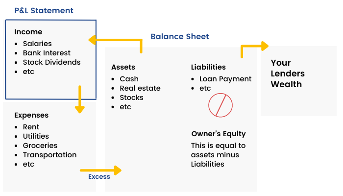
The major areas of Personal Finance can be divided into following parts –

1)Income

Income refers to the source of cash inflow for an individual. It includes Wages, Salaries, Dividend, Incentives, Bonus, Pensions, etc. This income can be spent to purchase essential and luxury commodities. It can also be used for savings and investment purposes. It is the first step in the Personal Finance Model.

2)Spending

It refers to the expenses incurred on buying goods or services. The common sources of spending are – rent, food, education, taxes, clothes, entertainment, etc. It is very important to manage one’s expenditure. If expenses are greater than the income, it may cause a deficit leading to borrowing of funds. Hence, managing expenses is a crucial part of the 'Personal Finance Model.'

3)Savings 

Savings refers to excess income over spending that is kept aside. The surplus between income and spending can be either saved or invested. The most common ways of keeping one’s savings are – Physical cash, Savings Account, etc. Individuals are advised to keep some money as savings to meet any short-term contingency. However, too much savings can lead to forgoing of high probable returns that could have been earned if the money was invested.

4)Investment 

Investment refers to purchasing of assets that are expected to generate a rate of return. It carries with itself an element of risk. Some forms of investments are Stocks, Bonds, Mutual funds, Real estate, Commodities, etc. There are different types of investment with various risk and return characteristics. Hence, it is very crucial to plan this.

5)Insurance 

Insurance is an agreement wherein a party (insurer) provides financial protection to another party (insured) in case of contingent, unforeseen, adverse event in future in return of premium. Various types of insurance include – Life Insurance, Health Insurance, General Insurance, etc.

Financial Model of a Company

Now that you have learned to build a financial model based on personal finance, it will be easier for you to grasp the concept of financial modeling at the company level. So let us dive into it.

A Financial Model on a company helps an individual to represent the business operation of that company using a spreadsheet. It is a summary of the overall business’s costs, income which can be used to make vital decisions in future. 

The flow would be -

There are three main financial statements that need to be studied for financial modeling.

• Income Statement 
• Balance Sheet
• Cash Flow statement

Income statement is the financial document that measures a company's financial performance over a specific accounting period. Financial performance is assessed by giving a summary of how the business earns and incurs its revenues and expenses through both operating and non-operating activities.

The purpose of the income statement is to show managers and investors whether the company made or lost money during the period being reported. It also contains the numbers most often discussed when a company announces its results - numbers such as revenue, earnings and earnings per share. It shows that at the end of the day, whether or not a business has generated any profits.

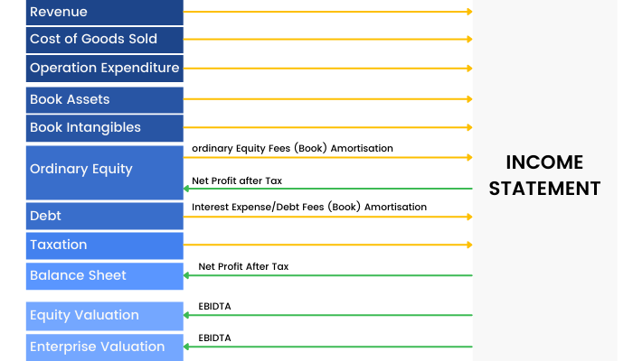
The layout of an Income Statement is governed by the accounting standards and reporting requirements applicable to each entity. It is also governed by the choices the entity makes (within the boundaries of its reporting requirements) as to how it structures the presentation of its revenues and expenses on its Income Statement.

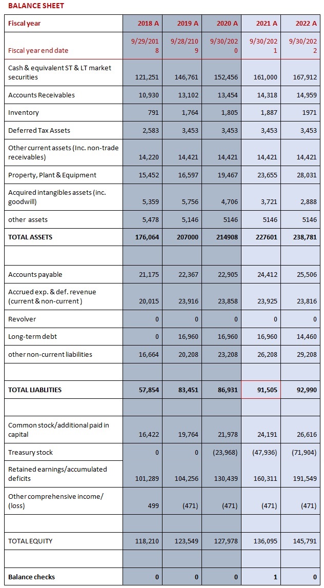
Balance Sheet highlights the financial condition of a company. It offers a snapshot of the company's health. It tells us how much a company owns (assets) and how much it owes (liabilities). The balance sheet is named by the fact that it represents a business' financial structure balances in the following manner:

Assets = Liabilities + Shareholders' Equity

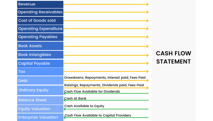
Cash Flow statement is a document which provides aggregate data regarding all cash inflows of a company from both its ongoing operations and external investment sources and all cash outflows on account of business activities and investments during a given quarter or year. It shows the true cash or liquidity position of a company. 

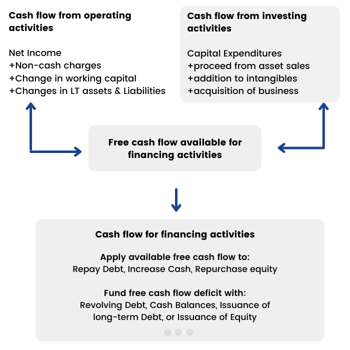
Companies produce and consume cash in different ways, so the cash flow statement is divided into three sections: cash flows from operations, financing and investing.

1) Cash Flow from Operating Activities (CFO) includes transactions from all the core or operational activities of a business. It shows how much cash comes from sales of the company's goods and services, less the amount of cash needed to make and sell those goods and services.

2) Cash Flow from Investing Activities (CFI) largely reflects the amount of cash the company has spent on capital expenditures, such as new equipment or anything else needed to keep the business going. It also includes acquisitions of other businesses and monetary investments.

3) Cash Flow from Financing Activities (CFF) describes the cash associated with outside financing activities. Sources of cash inflow would be cash raised by selling stock and bonds or by bank borrowings. Likewise, paying back a bank loan would show up as a use of cash flow, dividend payments and common stock repurchases.

Summarising the three Financial Statements – 

We can summarise the three financial statements in the following points – 

INCOME STATEMENT

• Keeps track of the revenue and expenses
• The top line is revenue, and the bottom line is net income after dividends
• It is also known as P&L (Profit and Loss) Statement.

BALANCE SHEET

• A record of the company’s holdings: its assets, liabilities, and equity at the end of the reporting period.
• It is a snapshot of the company over a time period.
• Total Assets = Total Liabilities + Shareholder’s Equity

CASH FLOW STATEMENT

• Shows how cash is being used during an accounting period.
• There are 3 categories – Cash from operating activities, Cash from investing activities, Cash from financing activities

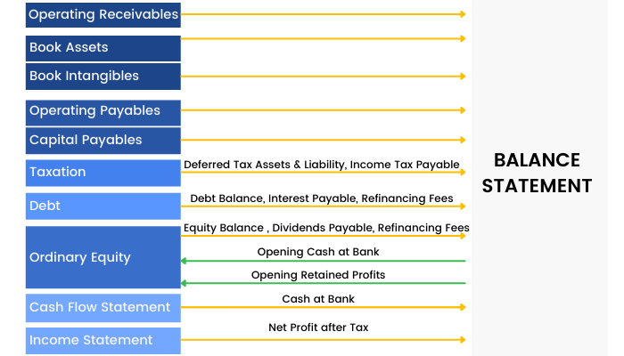
Flowchart of Interlinks Among the Three Financial Statements

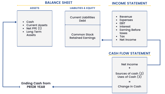
(1) PPE is Plant, Property & Equipment

(2) Sources of cash from decreases in assets or increases in liabilities between this year and prior year (e.g, sale of assets, new debt).

(3) Uses of cash from increases in assets or decreases in liabilities or equity between this year and the prior year (e.g, buildup of working capital, repayment of debt).

The Net Income that is calculated at the end of the Income Statement is used as the starting line item for the Cash Flow Statement. It is also transferred to the Retained Earnings account in the Liabilities side of the Balance Sheet.

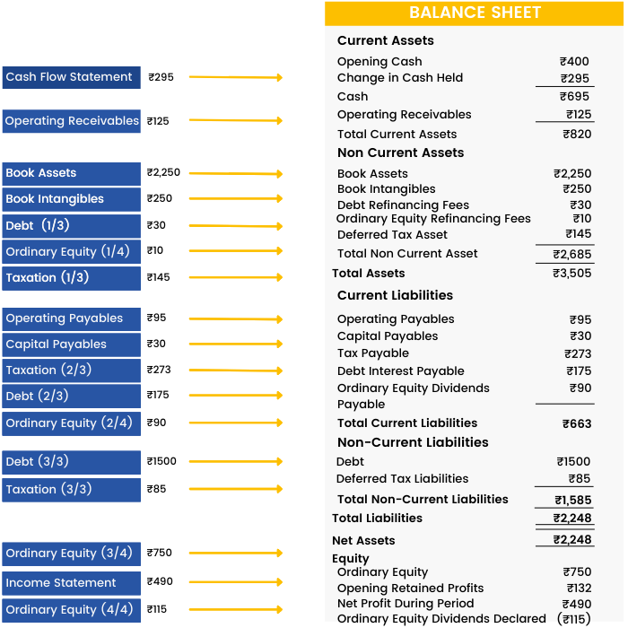
Another representation is as follows –

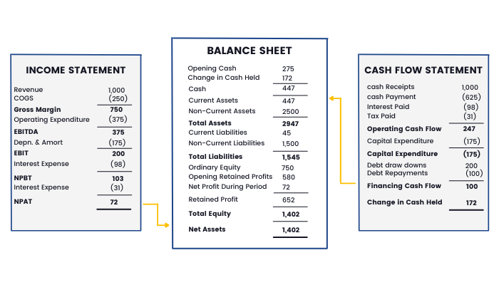
In the above figure, 

Net Profit After Tax (NPAT) of ₹72 from the Income statement is added to the Opening Retained Profits to calculate the Closing Retained Profits in the Balance Sheet. 

Changes in Cash held in Cash Flow Statement is the sum of Operating Cash Flows, Investing Cash Flows and Financing Cash Flows

₹172 = 247 + (175) + 100

This is added in the opening cash in the balance sheet. 

Approaches and Types of Financial Modelling

Previously we have learned to build financial models for personal finance and company finance. However, there are two different approaches and types in financial modeling. So let us discuss them in this section one by one:

1. Top-Down Approach 

In a top-down approach, an analyst examines the economic environment, identifies sectors that are expected to prosper in that environment, and analyses securities of companies from previously identified attractive sectors. It involves research driven market analysis - supply and demand analysis and competitor landscape analysis. 

In this approach, the company tries to assess its share of the pie and accordingly builds up its costs and revenue on a broad level.

• This is done by estimating the overall market potential for its product/service offering and then determining where it stands on the competitive level.
• In other words, the forecasts are initially developed at the brand, category or division level, and then allocated down to the lower levels.
• The overall expectations so determined percolate down to the value chain as specific targets for individual business units (profit centers). You can then plan and forecast sales and inventory requirements accordingly.

2. Bottoms-Up Approach 

In a bottom-up approach, an analyst typically follows an industry or industries and forecasts fundamentals for the companies in those industries in order to determine valuation. It involves fundamental business strategy analysis – core sales and marketing strategy and elasticity of product/service entry. 

• Individual activities and projects of a company become the focal point for planning action and operational managers have the freedom and flexibility to chart out their roadmap for the planning horizon.
• These individual figures are then aggregated to arrive at projected performance numbers for the company as a whole. 

Types of financial models

1.One-page DCF 

Comprises of less than 300 rows and gives you a ball-park valuation range, without much of granularity. Useful when you are making a pitch for potential acquisition targets and want to present a valuation range to your team members

2.Fully integrated DCF

• Forecasting revenue and cost of goods as per the segments and using price-per-unit and units-sold drivers instead of making an aggregate forecast. 
• Forecasting financials across different business units as opposed to looking only at consolidated financials
• Analyzing assets and liabilities in more detail

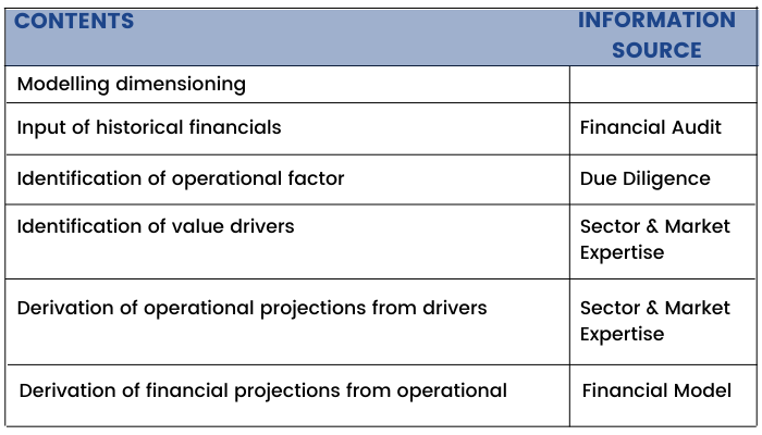
Steps to create a Financial Model

Earlier units have curated the idea behind financial modeling. However, there are some essential steps to keep in mind while building a financial model of a company. So, let us begin.

“History doesn't repeat itself - at best it sometimes rhymes” said Mark Twain.

The first step in creating the model is to get the historical statements in place, because this is what will give you a sense of where the company stands as on date. Historical parameters need to be adjusted for expected developments. While patterns could be discerned from the past it is not necessary that the future would be a replica of the past.

This exercise of analysing the historical Profit & Loss, Balance Sheet and Cash flow will impart a sense of realism to the financial model and make us forecast most pragmatically. 

As you start to build models, you will be wearing three hats:

• You are the finance expert, working with the elements of the financial statements
• You should be able to understand business dynamics and to forecast business performance
• You are the MS Excel wizard, optimising the available functionality
• You are the virtual architect, structuring a model that is transparent (easy to follow), flexible (easy to change), and robust (hard to break down).

Steps Involved in preparing a model

Step 1

A good financial model is simply a translation of business plan wording into numbers. Since this model becomes the financial roadmap of the company, all endeavour should be to capture the complexities of the business and generate streamlined and accurate data flows. The first step is to gather information on key parameters affecting the business which could be broadly as follows:

Understand as to what the cost and revenue drivers for the company are and what are the macro and microeconomic indicators which could have a bearing on the same.

For a petrochemical company, revenues, in terms of Gross Refining Margins (GRM) would vary substantially in line with international crude prices and the administered petroleum prices. 

Similarly, the EBITDA (Earnings before Interest, Tax, Depreciation and Amortization) margins for a company in the aluminium space would vary proportionately with the international/domestic prices of Aluminium Ingots, Bauxite and Electricity. 

Factors such as Inflation could have a more evident bearing on the fortunes of FMCG or Consumer Durables companies because their business model is based on tapping the surplus liquidity in the hands of an individual customer. All forecasts are assumptions (some of the major ones would be price, sales growth and cost of goods sold). The trick is to be reasonable and defendable while making them.

Step 2

For internal analysis business, understand the Cost Behaviour Pattern in terms of whether it is committed or variable.

For example, a company which goes into branding the goods sourced from Contract Manufacturers or engages labour force on contract basis would have lesser a burden of fixed overheads as compared to a company with in-house manufacturing facilities and a substantial number of people permanently on its payroll. 

An assumption made today that online advertisements would drive a company’s business revenues to USD 10 million by the year 2024 would be solely impacted by the variable factor called Click- Through-Rates. If the same is 0.1 per cent, therefore a website, which receives 100,000 page visits, would probably convert roughly 100 potential sales leads per ad campaign.

Step 3

Model the relations among parameters. They are usually linear relations, e.g. manufacturing 1 shirt, priced at ₹ 250 would require 2 meters of cloth purchased @ ₹ 50 per metre and entail an overhead expense of ₹ 75, but in some cases one may observe non-linear relations as well. In either case, establishing the relationship in an integrated manufacturing is not an easy task and one has to rely on past data and subject it to different statistical tests.

Step 4

Models ought to be dynamic. Sometimes things might not work the way you thought and hence reasonable models should provide flexibility to adjust to reality. 

Incorporate sensitivity analysis into the model in order to answer What if questions. For example,

What if the selling price of shirt falls down to ₹ 205 in the above example or the raw material costs go down to ₹ 40 per meter. The user must have the flexibility to vary each model parameter, one at a time or even more than one simultaneously and observe change in outcome (profit, break-even level) and also calculate Model Elasticity (percent change in profit/percent change in parameter).

Make the structure as flexible as possible so that one can change an individual module later on without changing the rest of the model. For example, the key output of the production module which is being taken to other sheets can be summarised at one place within the production module.

Thus, if required at a later stage, one can introduce the capacity expansion in the production module without having to change the rest of the model.

Step 5

Since each model parameter could vary in a given range, the model should also have a Scenario Analysis feature where the user is able to generate outcomes under the Best, Worst, and Most-Likely cases. This would help one to evaluate risk under alternative scenarios by measuring effects of possible parameter changes. Thus, the up-side and down-side risks of adopting a particular strategy would be clearly foreseeable.

Scenarios are feasible combinations of parameters:

Best case – Highest sales prices + lowest costs (only one possibility)

Worst case – Lowest selling price + highest costs (only one possibility)

Most-likely case – Most likely combination of prices and costs

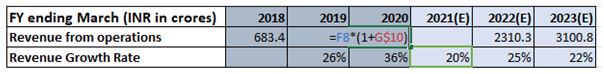
Let’s discuss how to forecast various elements – working capital, depreciation, amortization, etc. - that are linked to the financial statements in the end. We will discuss each element in our upcoming units.

Working Capital Schedule

Firstly, let us begin with the ‘Working Capital Schedule,’ which is a statement of change in the net working capital of a company. 

Working Capital – Steps 

• Create line-items - for example debtors, creditors, inventories, 
• Working capital items
• Reference the historical balances
• Project future working capital balances
• Calculate projected cash-flows
• Link to balance sheet and cash-flow statement

Working Capital Schedule - Assets

From the above schedule, we can notice that with an increase in the scale of operations and cost of goods sold, all the individual line items of working capital are increasing. Hence, year on year, we have to invest more and more in the working capital for the business. 

Working Capital Formula

Working Capital = Current Asset - Current Liabilities

(For financial modeling purposes - Current asset ignores cash; and current liabilities ignores revolver- which is overdraft facility)

Current assets on the balance sheet

• Trade receivables
• Short-term loans and advances
• Inventory
• Other current assets

How to Forecast Current Asset Items ?

Forecasting Trade Receivables

Assumption: We need to assume Receivable Days Outstanding. Receivables Days Outstanding is the average number of days it takes trade receivables to be converted in cash i.e., how long the company takes to collect cash from its account receivables.  

On the basis of this assumption and the forecasted sales amount the accounts receivable is calculated. Then, link these accounts receivable to the balance sheet.

Forecasting Inventory

Assumption: We need to assume Inventory Days Outstanding. Inventory Days Outstanding is the average number of days it takes the company to convert inventories into sales. 

On the basis of this assumption and the forecasted cost of goods sold amount the inventory is calculated. Then, link this inventory amount to the balance sheet.

Forecasting other items

• % of net sales.
• Can use historical data and project it into the future.
• These items are usually not a substantial amount as compared to accounts receivable and inventory.

Linking Working Capital to Balance Sheet

The highlighted region comes from the working capital schedule. 

WORKING CAPITAL SCHEDULE – (LIABILITIES)

Current Liabilities

• Create line-items
• Working capital items
• Reference the historical balances
• Project future working capital balances
• Calculate projected cash-flows
• Link to balance sheet and cash-flow statement

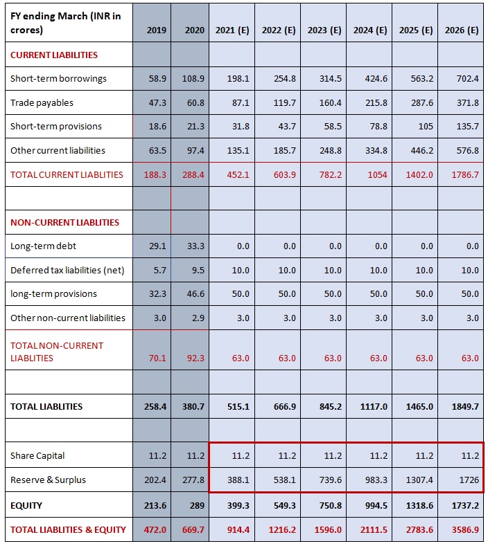
Current liabilities on the balance sheet are: 

• Trade payables
• Short-term provisions
• Other current liabilities
• Even short-term debt (also called as revolver) is a part of the current liabilities items, but it is forecasted later.

FORECASTING CURRENT LIABILITY ITEMS

Forecasting Payables

Assumption: We need to assume Payable Days Outstanding. Payable Days Outstanding is the average number of days a company takes to pay back its trade creditors/suppliers. 

On the basis of this assumption and the forecasted cost of goods sold amount the accounts payable is calculated.

Link this ‘account payable’ amount to the balance sheet.

Forecasting other items

For forecasting other items in the current liabilities section:

The most common way is: % of COGS

Can use historical data and project it into the future.

These items are usually not a substantial amount as compared to accounts payable.

Linking Working Capital to Balance Sheet

The highlighted region comes from the working capital schedule.

Linking Working Capital to Cash Flow

The highlighted region comes from the working capital schedule.

Illustrative Flow of Funds

Depreciation

Secondly, let us start with depreciation which is the loss in value of an asset over the period of its useful life.

What is Depreciation? 

• Depreciation is a method of allocating the cost of a tangible asset over its useful life of several years.
• Depreciation is a non-cash item.

In simple words we can say that depreciation is the reduction in the value of an asset due to usage, passage of time, wear and tear, technological outdating or obsolescence, depletion, inadequacy, rot, rust, decay or other such factors. 

Why Depreciate?

Depreciation helps in smoothing the income statement by allocating the cost.

Suppose a ₹500 asset is bought in FY 2010 which is going to be used for the next 5 years. It won’t be right to have ₹500 as expense in FY 2010; instead, the ₹500 should be spread over five accounting years (the useful life).

Depreciation is also used for tax purposes – as a way to lower tax expenses. Since it is a non-cash item, it does not reduce the cash balance of a firm, however, it helps in savings of the tax expense since the recording of depreciation will cause an expense to be recognized, thereby lowering stated profits on the income statement.

Depreciation Schedule

COMMONLY USED DEPRECIATION TECHNIQUES

Straight Line Depreciation

a)Simplest and most commonly used method.

b)Calculated by taking the purchase or acquisition price of an asset, subtracting the salvage value and then dividing by total useful years.

     Depreciation = (Cost of an Asset- Salvage Value)/Useful life

     Where,

• Cost of the asset is purchase price or historical cost
• Salvage value is value of the asset remaining after its useful life
• Useful life of the asset is the number of years for which an asset is expected to be used by the business

c)Depreciation is also used for tax purposes – as a way to lower tax expenses.

d)Produces a constant depreciation expense.

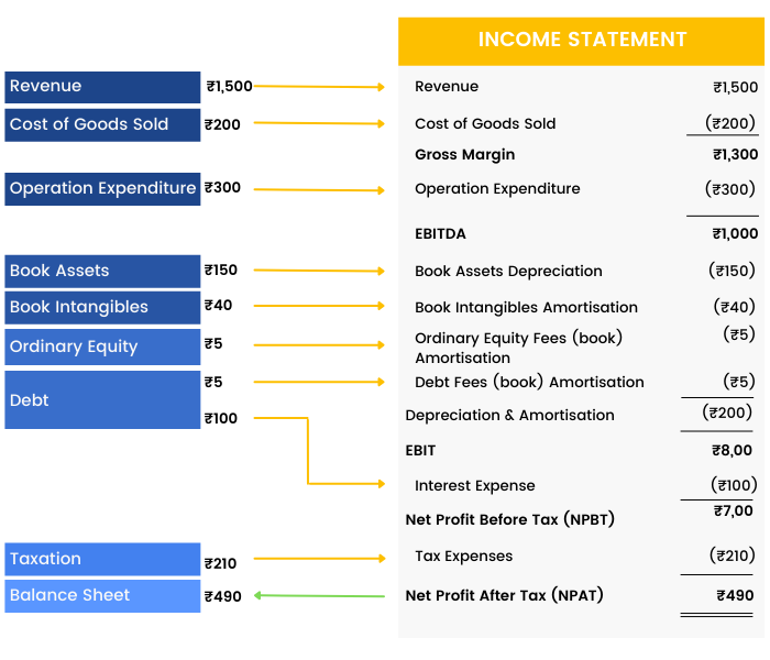
Example: - Consider an asset that costs ₹35,000 with an estimated useful life of 7 years and has a salvage value of ₹5,250. Under the straight-line method, the depreciation expense per year will be –

Depreciation expense = (35,000-5,250) /7 = ₹4,250 per year

Accelerated Depreciation

a)Allows companies to write off their assets faster in earlier years than the straight-line depreciation method and to write off a smaller amount in the later years.

b)It recognizes higher depreciation expenses during the earlier years as compared to the straight-line method of depreciation.

c)The major benefit is to provide a tax shield. In the initial years, the depreciation is higher as a result of which, tax charged on the profit is less compared to the later years. This results in deferment of tax liability since income in earlier years is lower. 

d) There are two popular methods – Double Declining Method and Sum of Years’ Digits Method.

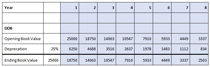
Double Declining Method – In this method, a fixed rate of depreciation is charged on the net value of the fixed asset at the beginning of the year. The rate of depreciation charged under this method is twice the rate that is charged under the straight-line method. The method reflects that assets are more productive in the earlier years as compared to their later years.

Depreciation Expense = 2 x Straight-line depreciation rate x Book value at the beginning of the year.

Example: - Consider a piece of property, plant, and equipment (PP&E) that costs ₹25,000, with an estimated useful life of 8 years and a ₹2,500 salvage value. To calculate the double-declining balance depreciation, set up a schedule:

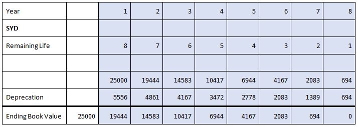
Sum of the Years’ Digits Method – In this method, the remaining useful life of the asset in a particular period is divided by the sum of the years’ digits. This fraction is then multiplied by Depreciable Cost. It recognizes depreciation at an accelerated rate. 

Depreciation Expense = Depreciable Cost * (Remaining useful life of an asset/Sum of Years’ Digits)

Where,

Depreciable Cost = Cost of asset – Salvage Value

Sum of Years’ Digit = n*(n+)/2, where n = useful life of asset

Example: - Consider a piece of equipment that costs ₹25,000 and has an estimated useful life of 8 years and a ₹0 salvage value. To calculate the sum-of-the-years-digits depreciation, set up a schedule:

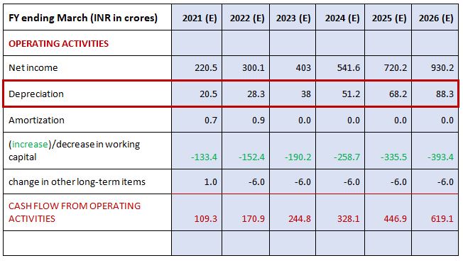
Depreciation & Cash-Flow Statement 

Depreciation is a non-cash expense.

Indirect cash-flow statements start with net income.

Net income includes depreciation expense.

Hence depreciation expenses are added back to Net Income to calculate the Operating Cash Flow.

Adding Back Depreciation 

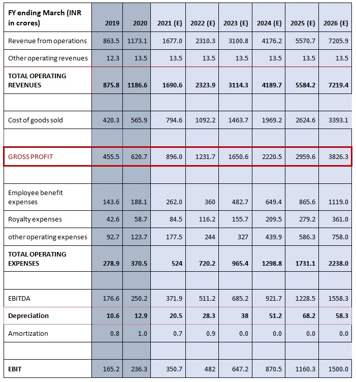
Depreciation & Income Statement

Depreciation expense is linked to the income statement below the EBITDA (Earnings before Interest, Taxes, Depreciation and Amortization) to calculate EBIT (Earnings before interest and taxes).

Linking Depreciation to P&L

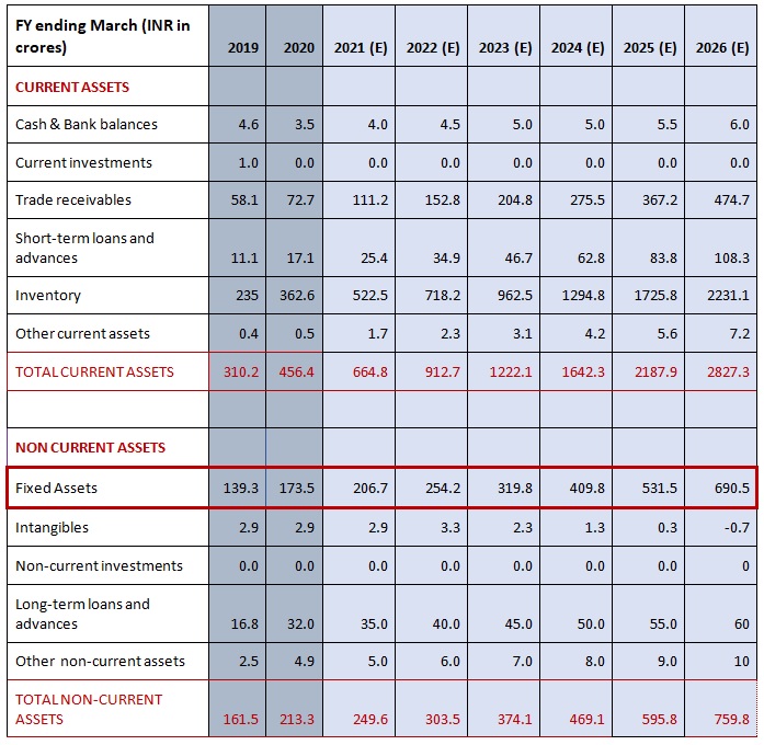
Depreciation & Balance Sheet

The ending property, plant, and equipment (PP&E) calculated in the depreciation schedule should be linked to the Balance Sheet.

Linking PP&E to Balance Sheet

The Fixed Assets in the Balance Sheet will be net of the depreciation for that year.

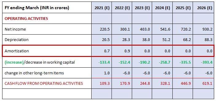
Amortization

Amortization is similar to depreciation that we learned in the last section. We have learned depreciation is the loss in value of tangible assets, whereas amortization is the loss in value of intangible assets. So, let us understand the concept of amortization.

What is Amortization?

Amortization is a method of allocating the cost of an intangible asset over its useful life.

Amortization is a non-cash item.

We amortize finite life intangibles like -

• Patents, slogans
• Capitalized software
• Deferred financing fees

For example, if Adani Group of Industries purchases software for its operational usage for ₹12 million, every accounting year, the company will expense ₹100,000 as amortization expense for 12 years, because software is an intangible asset.

Amortization expenses can be forecasted in several ways. The above shown is just one of the ways of forecasting amortization expenses.

Amortization & Cash-Flow Statement

Amortization is a non-cash expense.

Indirect cash-flow statements start with net income. Net income includes amortization expense.

Hence amortization expense is added back to the Net Income to calculate the Operating Cash Flow.

Adding Back Amortization

Amortization & Income Statement

Amortization expense in linked to the income statement below the EBITDA (Earnings before Interest, Taxes, Depreciation and Amortization) to calculate EBIT (Earnings before Interest and Taxes)

Linking Amortization to P&L

Linking Intangibles to Balance Sheet

The ending tangibles which we get from the Amortization Schedule is then linked to the Balance Sheet.

Long-term Items

There are several long-term items both on the asset & liability side of a company's balance sheet. In this unit, we will discuss the same. 

Other Long-Term Items Overview

• Use as a ‘catch-all’ for remaining balance sheet items
  - Long-term items without drivers
• Create line items
• Reference historical balances
• Forecast balances
  ​- Keep balances constant if drivers are not easily recognizable

Long-Term Items

Asset side 

• Long-term loans and advances
• Other non-current assets
• Deferred tax assets

Liability side

• Deferred tax liability
• Long-term provisions
• Other non-current liabilities
• Forecasting Future Balances

Deferred Tax Assets (DTA) and Deferred Tax Liabilities (DTL) are for temporary differences between your taxable income as per the Companies Act and taxable income as per the Income Tax Act. If you are paying more tax today but pay less tax in future, then you will build Deferred Tax Assets. If you are paying less tax today but have to pay more in future, then you will build Deferred Tax Liabilities.

• Keep long term items constant for projected years if you have no drivers.
• Usually, these items will have no drivers.
• When projecting, never input the numbers – always link to historical numbers. These are also called flat lined references. It is just linked to the actual historical financials.

Linking Other Long-Term Items

• Once the schedule is set- calculate cash flows on the basis of changes in long-term items.
• Link the change to the cash flow statement.
• Link the ending amount of forecasted other long terms items to the balance sheet.

Other Long-Term Items & Cash-Flow 

Other Long Term Items & Balance Sheet 

Other Long Term Items & Balance Sheet 

Things to Remember

Other Long-Term Items Schedule is just a catch all category.

There’s very little that an analyst can know or forecast about other long-term items and hence usually it is flat-lined and kept constant.

Shareholder Equity

Let us start with shareholder's equity now. 

Equity Schedule

• Project shares outstanding
• Reference back to historical count (flat-line)

Purpose: Need EPS (Earnings Per Share) for share repurchase

• Will factor in share repurchase later
• Calculate remaining line items:
• Leave interest expense / income blank
• Will complete later with interest  schedule

A Simplified Equity Schedule 

Equity Schedule – Overview

Setup:

• Line-items
• Input selected historicals

Project:

• Share repurchase, option proceeds, and new shares from exercises options
• Dividends and future equity balance
• Full blown Equity Schedule Items and Flow

Flow of equity schedule:

Beginning equity balance

Add: Net income

Add: Issuance of shares

Less: Repurchases

Less: Dividends paid

Less: Options Proceeds

Add/Less: Effects of exchange rates on cash

Share repurchase assumptions

1. Flow of share repurchase assumptions:
2.Current year EPS
3.Assumed current year EPS multiple
4.Project share price
5.Project shares repurchased
6.Multiply (3) and (4) to calculate the rupee amount in shares repurchased

ESOP (Employees Stock Ownership Plan) related assumptions

Treasury Stock Method (TSM)

a)The net of new shares that are potentially created is calculated by taking the number of shares that the in-the-money options purchase.
b)Then subtracting the number of common shares that the company can purchase from the market with the option proceeds.
c)This adds to total number of shares and lower EPS in future years.

Linking Equity Schedule

Link ending balances calculated in the shareholder’s equity schedule to the balance sheet.

Link repurchases, options, dividends to cash flow statement.

Equity Schedule & Cash-Flow

The highlighted region comes from the Equity schedule.

Equity Schedule & Balance Sheet

Calculating Shares Outstanding

1)Enter historical share information:

• Basic shares: actual and average
• Effect of options
• Diluted shares: average

2)Reference repurchases shares and new shares from exercised options:

• Calculate projected basic shares (actual)
• Calculate average basic and diluted shares
• Reference projected shares to Income Statement

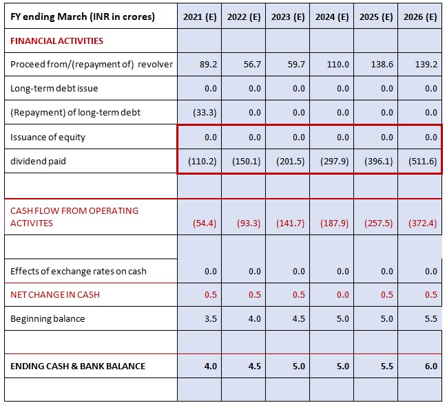
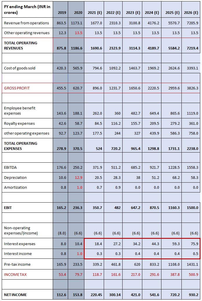
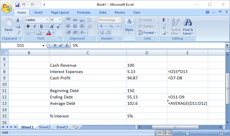
Debt and Interest

Debt & Interest are also an important part of a financial model. So let us discuss both of them in this unit. 

Debt and interest Schedule (Part A)

Debt and interest Schedule (Part B) 

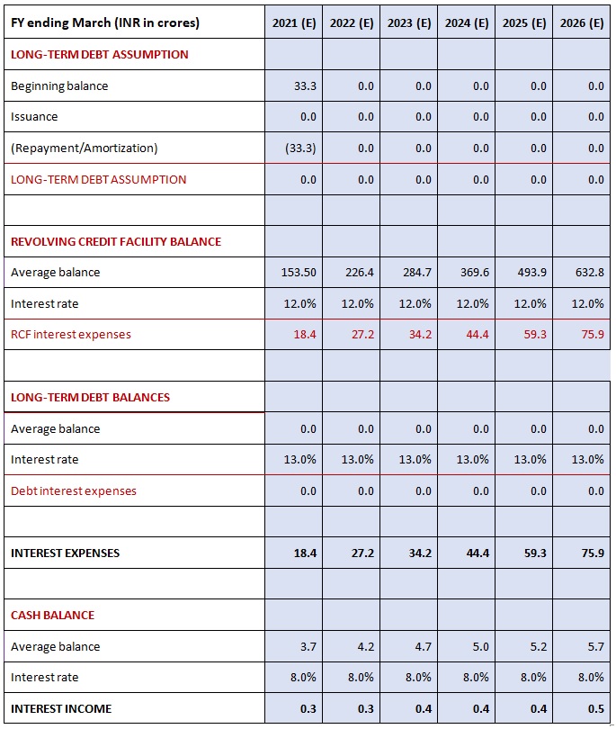
Average Balance = 0.5 (Beginning Balance + Ending Balance)

Progression of the Cash Flow

Preparing for Debt and Interest

a)Income statement: missing interest expense / (income)

b)Balance sheet: missing cash and debt items

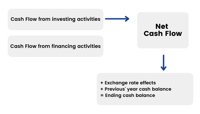
c)Cash-flow statement:

• Calculate cash flow from operating and investing activities.
• Calculate cash flow available for financing activities.
• Calculate ending cash balance.
• Link with balance sheet.
• Cash flow from operating activities

Steps

Link net income to the cash flow statement.

d)Calculate CFO, CFI, and CFF.

e)Calculate CFF and net change in cash.

f)Reference beginning cash balance from the balance sheet and calculate ending cash balance.

g)Link ending cash balance to the balance sheet.

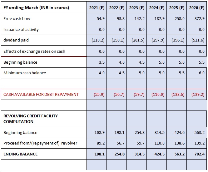
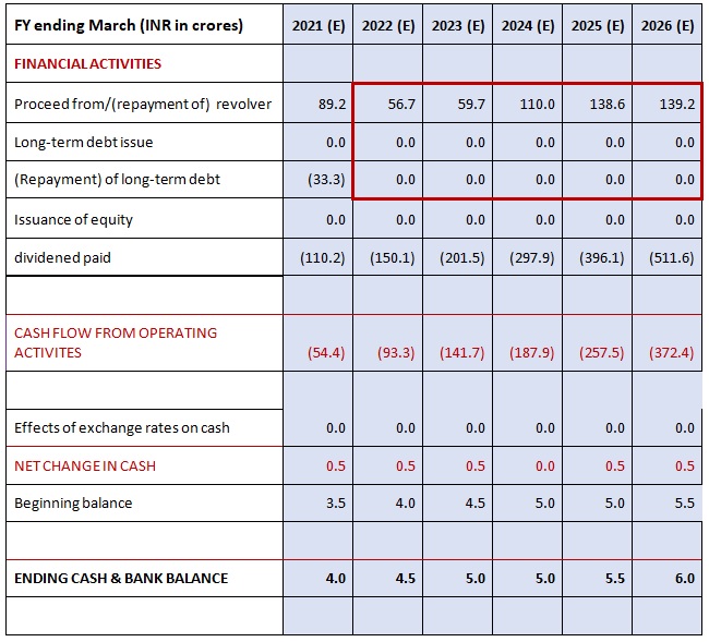
Debt and Interest (Overview)

Cash Flow available for debt repayment

Long term:

a)Reference in historical balances

b)Enter mandatory long-term debt repayments

c)Calculate projected long-term balances

Calculate – Cash flow available for revolver

Revolver = Cash sweep 

Cash sweep refers to using the company’s excess cash flows to pay off the debts.  

Calculate interest expense / (income)

• Based on average balances
• Revolver interest expense
• Long-term debt interest expense
• Cash balances for interest (income)

Linking Debt Schedule

Link:

• Projected interest expense / (income) to income statement
• Projected debt repayments / borrowing to cash flow statement
• Projected debt balances to the balance sheet

Debt Schedule & Cash-Flow 

The highlighted region comes from the Equity schedule.  

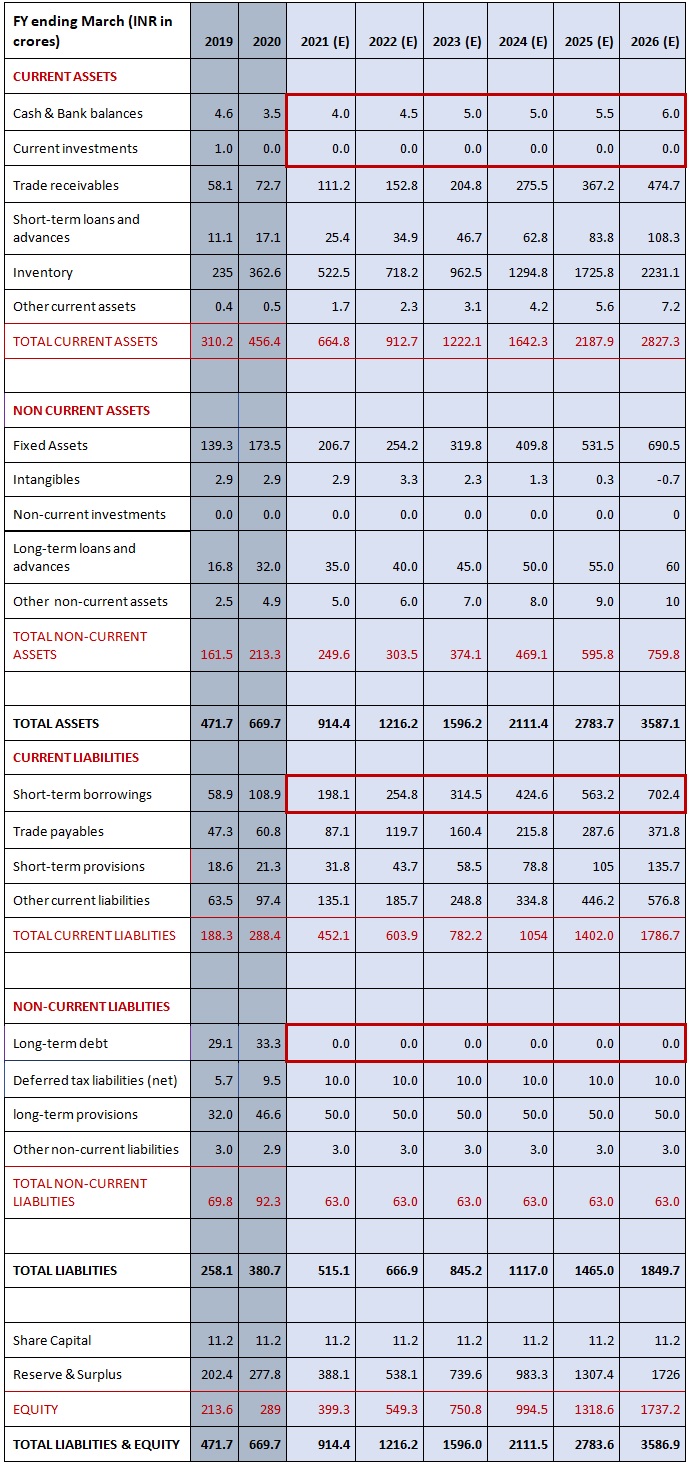
Debt Schedule & Balance Sheet

Guidelines for Creating an Effective Model

Earlier, we have learned various elements & their importance in financial modeling. But it is essential to have proper guidelines to create an effective model. The following points must be taken into consideration while creating a financial model:

1. Documentation

Ensure the model has adequate documentation so that it can be easily modified later. The documentation would help in understanding the design and structure of the model and would be particularly useful when the model is required to be operated by a person other than the person who has developed it. Every financial model would have multiple worksheets and calculations. To help users understand the model, one can put a schematic diagram on the front sheet of the model for describing the various sheets and indicating how they interact with each other. One can also use hyperlinks to the relevant modules, thereby making the first sheet as a navigational tool, helping users to find their way around.

2. Input Tabs - Assumptions

All of the model’s hard-coded assumptions such as revenue growth, WACC, operating margin, interest rates, etc. should be kept in a clearly defined section of a model — typically on a dedicated tab called ‘inputs.’

The user has only one place they need to go to change any assumptions. This creates a consistent distinction between areas in the model that the user works in vs. areas the computer works in.

The flow thus would be 

Assumptions → Calculations → Output

3. Hardcodes = landmines

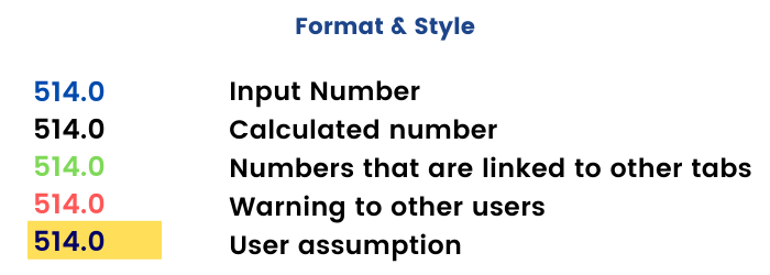
Please take an oath that you will never put a hardcode and a formula in the same cell. All hardcodes or “inputs” should pull out of formulas and consolidated in an inputs / assumptions section. Never repeat an input and you can assign a specific colour to it so you can find them easily.

The danger here is that you’ll likely forget there is an assumption inside a formula. Inputs must be clearly separated from calculations

This hides the information that the PAT Ratio is 65%, but more critically, it means extra work if you need to change the PAT Ratio later, since you will have to go to the individual cells (assuming that you remember where all the hard-coded 60% entries are).

So, never embed inputs in formulas.

Instead, break out into separate line items

4. Going Circular (References)

Circularity refers to a cell referring to itself (directly or indirectly). Usually, this is an unintentional mistake. In the simple example below, the user has accidentally included the sum total (D5) in the sum formula. Notice how Excel becomes confused:

Avoid it if you can. If you have to do it, fine, but check the “enable iterations” box and build in a “circuit breaker” or be prepared for a lot of #REF!

But sometimes a circularity is necessary. Let’s say, if a model calculates a company’s interest expense based on a cell that calculates the company’s revolving debt balance, but that revolving debt balance is itself determined by (among other things) the company’s expenses (including interest expense), then we have a circularity:

The logic of such a calculation is sound: A company’s borrowing needs should take into account the interest expense.

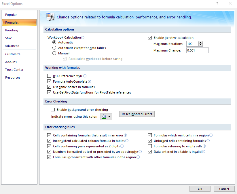
Intentional circularity in financial models need a special setting must be selected within ‘Excel Options’ to prevent Excel from misbehaving when a circularity exists:

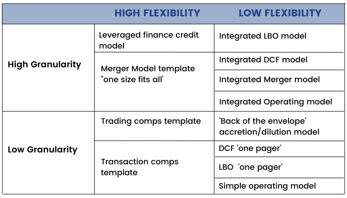
5. Granularity - Bottom Up

The devil lies in the details. And for the financial model to have its appeal, it should always follow a bottom up approach to building items such as revenue and cost. Unless you demonstrate that the model captures the complexities of the underlying business, it will simply remain a complex sheet of MS Excel with little relevance to the end user. 

Consider the case of a pizza store. Monthly sales could be the result of the following inputs: foot traffic per day, days open per week, conversion rate per customer, average order quantity, and price per pizza. To a reasonable extent, the more granular your model, the more accurate and defensible it’s likely to be.

6. Financial model flexibility

A model’s flexibility stems from how often it will be used, by how many users, and for how many different uses. A model designed for a specific transaction or for a particular company requires far less flexibility than one designed for heavy reuse (often called a template).

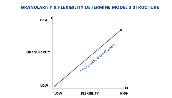
Together, granularity and flexibility largely determine the structural requirements of a model. Structural requirements for models with low granularity and a limited user base are quite low. Remember, there is a trade-off to building a highly structured model: time. If you don’t need to build in bells and whistles, don’t. As you add granularity and flexibility, structure and error proofing become critical.

7. Present ability

Regardless of granularity and flexibility, a financial model is a tool designed to aid decision making. Therefore, all models must have clearly presented outputs and conclusions. Since virtually all financial models will aid in decision-making within a variety of assumptions and forecasts, an effective model will allow users to easily modify and sensitize a variety of scenarios and present information in a variety of ways.

8. Link directly to source cell

Always link directly to a source cell as it is more difficult to audit “daisy chained” data 

9. Build in error checks

The most common error check in a financial model is the balance check — a formula testing that assets = liabilities + equity should be employed.

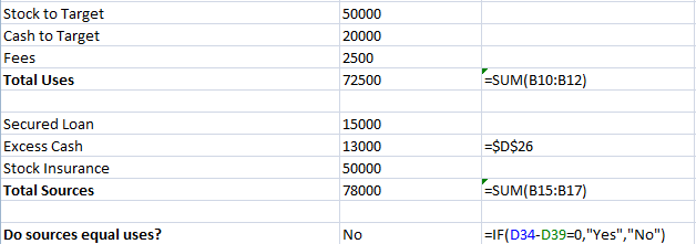
So have checks like ensuring sources of funds = uses of funds 

Similarly, you could ensure that total forecast depreciation expense does not exceed Plant, Property & Equipment (since depreciation is the wear and tear of (PP&E.) or that debt repayments does not exceed outstanding principal.

Use as many control checks (for example, total assets = total liabilities, sum of product mix =100 %, opening stock + production/purchases - sales - closing stock = 0, etc.)  as possible to ensure that there is no conceivable error in the model. Also, they should be built in such a way that they automatically flash whenever an error occurs in the model. It would also be a good idea to familiarise oneself with the advanced features of Excel and frequently using them, for example, the data validation feature avoids the accidental selection of incorrect value for an input cell.

10. Ruler Testing Your Model

The following points must be taken into consideration for testing your model: -

a) A balanced model doesn’t mean a correct model
b) Go line by line through your model
c) Are your assumptions reasonable and defensible?
d) Is everything properly formatted?
e) Have you footnoted appropriately?
f) Hand check each and every calculation

Scenario Analysis

After successfully creating a financial model, it is essential first to analyze then make a decision. The process is called scenario analysis. Scenario Analysis is also known as “What-if” Analysis. It can help you to gain better confidence in projections.Scenarios are feasible combinations of parameters:

• Best case – Highest sales prices + lowest costs (only one possibility)
• Worst case – Lowest selling price + highest costs (only one possibility)
• Most-likely case – Most likely combination of prices and costs

Common Uses of Scenarios –

• Allow for sensitivities analysis
• Able to better answer “What if” questions
• Gain better confidence in projections
• Varying levels of operating performance
• Range of synergy realization
• Multiple target analysis in Mergers and Acquisitions (M&A) situations
• Stress test for loan structuring and covenants

Various Sources for Scenarios –

• Management forecasts
• Internal budget or forecasts
• “Outlook section” in the MD&A
• Research expectations
• Based on historical performance

One should always play around with assumptions to see if they make sense in all cases. The assumptions must be reasonable and defensible.

Case Study – ITC Limited

To find out a stock's intrinsic value, financial modeling is useful. So let us find a stock's intrinsic value with the help of a case study.

Let’s calculate the Present Value of ITC Limited using DCF Analysis.

Before diving into the calculation, let’s first understand the method of Discounted Cash flow Analysis.

 Discounted Cash flow Analysis (“DCF Analysis“) is a widely used method of stock valuation. The goal of DCF Analysis is to estimate the amounts and dates of expected cash receipts which the company is likely to generate in future and then arriving at the present value of (the sum of) all future cash flows using an appropriate discount rate.

Discount rate is the minimum rate of return, which the investor expects from the investment.

Discount Rate = opportunity cost = desired return on investment. In other words, “The value of any investment is the discounted present value of all its future cash flow

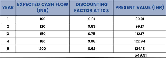
Discounting Factor is a weighing factor that is used to calculate present value of future cash flows. It is calculated in the following way –

DF = (1+r) ^ (-n)

Therefore, we can calculate the present value for each year’s expected FCF and add them up. Use the formula below to do this.

Present Value = FCF/ (1+r) ^ n, where r = discount rate

 So, let us say there is a company where cash flows forecasted over the next 5 years are as follows:

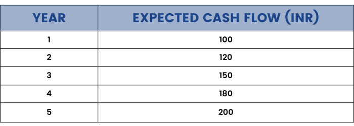
Let us calculate the present value, using a discount rate of 10%.

Thus, if the stock is available at INR 500, it is a bargain.The stock is undervalued (i.e., Present Value > Market Value) and before the market realises it, we must buy it.

The most important, yet difficult aspect of DCF analysis is the projection of future cash flows and future capital expenditure. To do a meaningful analysis, you need at least the previous 5 – 10 years of data and projections for a similar period in future. Also, the DCF method requires a large number of assumptions. Hence, the model is very sensitive to changes in assumptions.

Nevertheless, it is an important and famous method of equity valuation.

So now, let us calculate the present value (you may call it the intrinsic value) of ITC Limited using the DCF Analysis model.

The formula for calculating the Present Value would be:

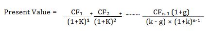
The formula we use looks somewhat complicated on paper but is extremely easy to use once you have assumed all values

PV = Present Value

CFi = Cash Flow in year ‘’' (i.e. CF1…CF2….CF3….till CFn-1)

k = Discount rate

g = growth rate assumption in perpetuity beyond terminal year

n = the number of periods in the valuation model including the terminal year

Therefore, we follow the following steps -

Step 1: Determining the Revenue Growth Rates

Growth Rate: Growth Rate is the rate at which a company is expected to grow in the future. You have to be very realistic and rational about the growth rate you chose for the company, else the intrinsic value arrived may be misleading.

You can estimate the growth rate of a company by looking at the past earnings growth record or by reading the reports by various analysts and make a consensus growth estimate.

Based on the past and expected future performance of both ITC and the economy, we can project the growth rate of revenues -

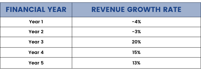
Therefore, we have assumed that ITC will grow at 4%, -3%, 20%, 15% and 13% over the next 5 years. 

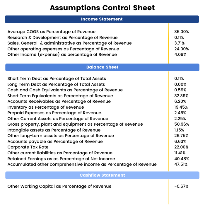
Step 2: Forecasting the Financial Statements

Now, based on financial statements of the last 5 years, we computed different ratios for ITC Limited, across financial figures in the P&L Account, Balance Sheet and Cash Flow Statement. 

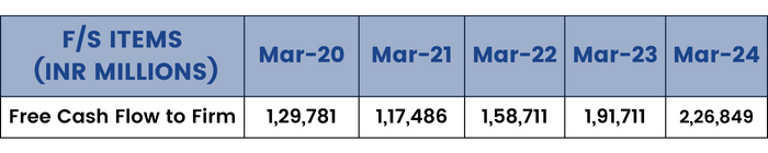
Step 3: Deriving the FCFF 

Free Cash Flow: Free cash flow is the cash left with the company after paying for all the expenses related to daily operations of the business and any assets bought to expand the business(such as plant and machinery).

Free cash flow is the most important and reliable part of Discounted Cash Flow (DCF) analysis because unlike Net Profit and sales, which are prone to accounting manipulation and window dressing, cash flow statements are hard to manipulate. 

Free cash flow of the company can be calculated using following formula:

Free Cash Flow = cash flow from operating activities – capital expenditures

Note – Cash flow from operating activities indicates the net cash flow a company earns from its regular business operations, such as manufacturing and selling of goods and services. Capital expenditure is the money used for purchasing or maintaining physical assets like property, plants, machines, etc. 

This is the trickiest part as projection is based on pure assumptions you make about the future of the business. It is always intelligent to be slightly conservative so that you do not overpay for a business.

Step 4: Calculating the Terminal Value

Terminal value (TV) is the value of a business or project beyond the forecast period when future cash flows can be estimated. It assumes that a business will grow at a set growth rate forever after the forecast period. Terminal value often comprises a large percentage of the total assessed value.

The formula to calculate TV is –

TV = FCF *(1 + Growth rate)/(Cost of capital – Growth rate)

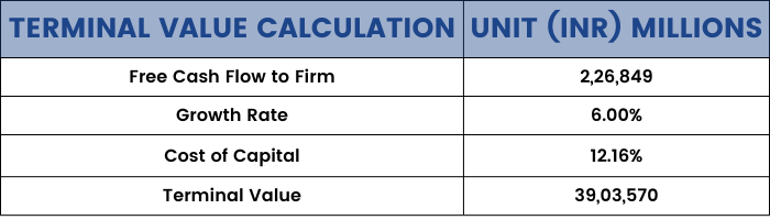
Remember that Growth Rate represents an assumption that a company will continue to grow at a steady constant rate into perpetuity at 6% p.a. 

Typically, the perpetual growth rate ranges from historical inflation rate to historical GDP growth rate.

Step 5: Calculating the Discount Rate

DCF analysis helps assess the viability of a project or investment by calculating the present value of expected future cash flows using a discount rate. Here we use the Weighted average cost of capital (WACC) to discount the cash flow. WACC is the cost of capital in which each type of capital (equity, debt) is weighed proportionately. The below table from the excel model shows the calculation of WACC for ITC Valuation.

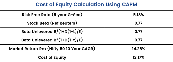
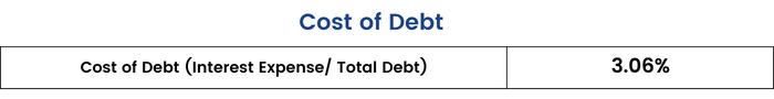
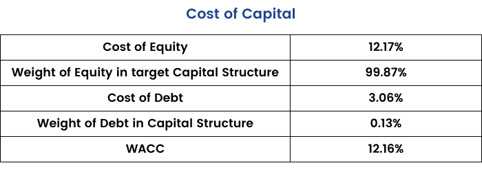
WACC = Cost of Equity*Weight of Equity + Cost of Debt*Weight of Debt

= 12.17*0.9987 + 3.06*0.0013 = 12.16%

Discount rate is usually calculated by using CAPM (Capital Asset Pricing Model) method, which calculates the weighted average of cost of capital of both debt and equity. Thus, we will discount the cash Flows at 12.16% 

Step 6: Discounting the Cash flows

The WACC and the Cost of Equity for the company calculated in the above step are then used to discount the FCFF and Terminal Value calculated in Step 3 and 4. 

In our case, we’ll only consider the FCFF based Intrinsic price of the shares as it represents the cash flow to all the suppliers of capital and not only to the equity shareholders. Thus we arrive at the Present value of future FCFF for ITC Valuation. (Units are INR Millions)

We find the discounted market capitalization of the company, which is the sum of present value of all the future cash flows and perpetual present value.

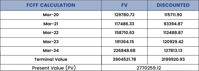
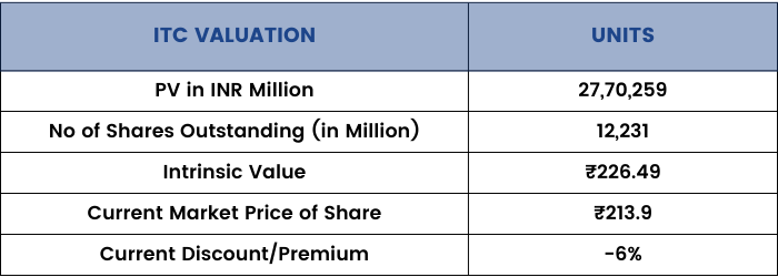
Thus, by applying the growth rates, we come to a calculation that the Present Value of the Cash Flow available to the firm is INR 27, 70,259 million. 

Step 7: Arriving at the Intrinsic Value of the Shares

Dividing the PV of the FCFF and Terminal Value (the Value of the entire firm) by the number of outstanding shares we get the per share intrinsic value. We can compare this price with the current market price of the stock to understand whether the stock is overvalued or undervalued, whether the stock is trading at discount or premium. 

• If the Intrinsic Value of Share > Market Value of the Share, then the stock is undervalued – one should buy the stock. 
• If the Intrinsic Value of Share < Market Value of the Share, then the stock is overvalued – one should not buy the stock, rather should sell the stock if in possession. 

Future is anything but predictable. Always remember, "your predictions will more often be wrong than right" so give yourself a margin of safety (i.e. margin to go wrong). In other words, buy stocks, which are available far below their fair or intrinsic value.

Conclusion

So we have finally at the end of this module where we got a detailed explanation about the uses of financial modeling and its importance in stock analysis. There are more such types of modules on ELM School that offer knowledge on stock analysis and other areas of finance.